Time-Series analysis for wind speed forecasting

(1)

https://doi.org/10.26637/MJM0S01/11

Time-Series analysis for wind speed forecasting

Garima Jain

1

Abstract

In this paper, an enormous amount of study has been made on various weather forecasting models and many specialists developed different models for optimal results. Different models which is taken for implementation and were used for predicting the forecasted data. A technique used for forecasting the given data is defined as a time series data. Box-Jenkins method is a statistical methodology used for prediction of data in time series. During this paper, an ARIMA model is implemented for predicting the data of Wind Speed. Results are compared with respective model i.e.., ETS Model. With this paper we like to through some light on ARIMA (Auto-Regressive Integrated Moving Average) and ETS (Exponential Smoothing) models for forecasting the weather conditions in India. ARIMA model is chosen; because of it is acceptable in terms of easiness and extensive of the model. Eight years weather data (from year 2007 to 2014), i.e., wind Speed for time-intervals to forecast (i.e.., 1 hours) are used in this research.

Keywords

ARIMA (Autoregressive Integrated Moving Average), ETS (Exponential Smoothing), AIC (Akaike’s Information Criteria), BIC (Bayesian Information Criteria), RMSE (Root Mean Square Error), Mean Absolute percentage Error (MAPE), Mean Absolute Error (MAE) and Box-Jenkins.

1_{Department of Computer Science and Engineering, Swami VivekanadSubharti University, Meerut-250005, India.}

*Corresponding author:1_{jaingarima2011@gmail.com}

Article History: Received24December2017; Accepted21January2018 c2018 MJM.

1. Introduction

Wind speed has as of late gotten an expanding consid-eration around the earth due to its inexhaustible nature and also ecological agreeableness. The distinctive advantages of wind vitality are joined by a few difficulties: high capri-ciousness, restricted likelihood, constrained dispatchability and non-storability. Climate determining is an arrangement worried about future climate. Weather forecasting concerned with various strategies which make use of relativelysimple observation of the sky to advance computerized mathematical Models [5]. Application like ARIMA has one of the impor-tant uses in time series prediction another or equal technique

to the traditional statistical strategiesthat are utilized in the prediction of time-series like MA, AR and ETS Box-Jenkins models [1]. These ancientstrategiesare generally known as Time Series strategies. However, meteoricknowledgeis unsure (uncertain) in nature and data on weather is mistilyoutlined [3]. Predicting weather has always been a difficult field of research analysis with a very slow progress rate over years. Weather data consider the noises and outliers therefore; the investigation may not be accurate. Random error is defined as noises (or bug) that comes from the device network, error writ-ing and so on. Weather forecastwrit-ing is a crucial issue within the field of meteorology all over the world. Weatheris taken into accountbecause the most difficultdrawback witnessed by the globewithin the last decade. The use of wind energy has been developed considerably throughout the world, in order to get the ideal for the future with electricity without pollution. Wind is one of the weather variables which are very difficult to predict. In wind power forecasting, there are two approaches commonly used [6].

(2)

in large uncertainties of wind speeds. Extensive efforts have been dedicated to develop efficient wind speed forecasting models. Recent advances toward a better understanding of the hydro dynamical aspects of the difficulties, coupled with-the development of high-speed computing tools, promise to createthe current area one amongst the foremost exciting in all meteorological history [1]. Instead of requiring separate power forecasts, they can get them by converting the com-mon wind speed forecasts based on their own power curves. Wind speed forecasting can be more precise than wind power forecasting due to the spatial correlation of wind. Instead of demanding separate power forecasts, they can usually get them by transforming the common wind speed forecasts.

A. Objective

One of the recent objective of the weather study is to im-plement a method that generated an improving idea about the forecasting approximation of different parameters. There are number of struggles which should be made to develop and improve the existing time series weather forecasting models by using different techniques. The role played by statistical methodology for forecasting the weather parameters is defined to be most important for their detailed estimates. The original measurement time-series comprises 54,956 data correspond-ing to wind speed in nautical-miles per hour (kn), acquired each 1 hour.Kn is a symbol which is illustrated as a ISO Stan-dard. The knot is defined as a unit of speed which is equal to one nautical mile as 1.852 km (or 6076.12 feet) per hour, approximately 1.151 mph internationally which means that 0.0639% should be added to “UK knots” to get “International Knots”.

Weather Data of India from the dates May 03, 2007 to March 06, 2014 was used to provide useful insight about the performance of the algorithms. The recorded data of the years 2007-2014 were used to make predictions. The accuracy of various models is measured and then compared by Moving Absolute Error, Moving Absolute Scaled Error, Moving Ab-solute Percentage Error and Root Mean Square Error. We also include the criteria Akaike’s Information Criteria and Bayesian Information Criteria. The model which formed the best prediction result will use for comparison and prediction. In this paper, ARIMA model is used in R software for pre-dicting the weather. R is widely used Language not only by scientists but also in many time series applications. It is an additional concept including mathematical and statistical ex-pertise which helps us to groom our knowledge in analytical field that when deployed into existing processes makes them adaptive to improve conclusions [4]. Thus, together with these advantages offered by this software, we can predict the results before they occur. ETS model is also used from R Software with R Studio Tool. These tools apply R techniques to data modeling. This allows our stationary analytical systems to learn from the data they are modeling [5]. These methods are defined briefly by Hyndman and Khandakar (2008) collection of functions for evaluating time series data, as well as many

more interesting time series datasets for different functionality. The package Forecast (Hyndman, 2010) provides additional care for forecasting using ARIMA and an extensive class of exponential smoothing models.

The data are collected from the Indian Meteorological Department which is the head office. In the data set, there we have Wind Speed parameter measurements, and this data are only on Indian weather condition. For analysis and forecast, we applied ETS and ARIMA on this data; finally they are evaluated and compared.

B. Outline

The rest of the paper is organized as follows: Section 2 describes the conceptual study on ARIMA model. Section 3 is used for approaches named as ETS model and data demon-strations, the models that are examined are also described in Section 3. Section 4 presents and analyzes the results. Finally we summarize and give future direction of research in Section 5. Section 6 describes the related references.

2. ARIMA

ARIMA stands for Autoregressive Integrated Moving Av-erage. ARIMA models aim to define the autocorrelation in the parameter value and can be applied to evaluate stationary and non-stationary time series. ARIMA model is the technique which is implemented and designed by the respectable Box and Jenkins (1976). It is an optimal combination of three de-signed calculated models. It uses auto-regressive, integrated, moving-average (ARIMA) models for time series data. The

model is known by ARIMA(p), where p≥0. After

differ-encing ARMA Model finitely many times we correspond to

an ARIMA Model. The componentspandqare defined as

the order for AR and MA parts, whereasd is the degree of

differencing. Differencing is generally used to eliminate the trend (may be linear or exponential) in a time series. The differencing orderdrelates to how many times the processYt

requests to be differenced to become stationary. To see that if the Time Series is Stationary or not we take help of ACF (Auto Correlation Function) and PACF (Partial Auto Correla-tion FuncCorrela-tion). Time series is a set of interpretaCorrela-tions ordered (sequentially) according to the time they were observed.

An ARIMA(p,d, andq)model can explain for temporal dependence in several ways.

• First, the time series is taken to reduce it stationary, by taking d differences. Ifd=0, the observations are modelled directly, and in case, ifd=1, the differences between successive observations are modelled.

• Second, the time that depend on the stationary process is modelled, by including p Auto-regressive (AR). The equation forpis that:

Yt=c+ϕ1Yt−1+ϕ2Yt−2+· · ·+ϕpYt−p+Zt,

(3)

where, c is an unknown constant term, and ϕi, i=

1,2, . . . ,p, are the parameters of the AR model.

• Third,qis related as the moving-average terms. It takes the observation of previous errors. The equation forq

is that:

Yt=c+Zt+θ1Zt−1+· · ·+θqZt−q, (2.2)

where,cis an unknown constant term, andθ1, . . . ,θq,

are parameters of the MA model.

• Finally, combining these three mathematical models

we get ARIMA model. So the integrated form of the ARIMA model is that:

Yt−1=a0+ (1+ϕ1)Yt−(ϕ1−ϕ2)Yt+1−p

+ϕpYt−p+θ1Zt+· · ·+θqZt+1−q+εt,

(2.3)

where,Yt, a stationary is a stochastic process, a0 is

the constant,∈tis the error or white noise disturbance

term,ϕpmeans auto-regression coefficient andθqis the

moving average coefficient. If we consider a cyclical time series, following steps can be repeated according to the period of the cycle, it may be viewed whether quarterly or monthly or other time interval. ARIMA models result in extremely flexible for continuous data analysis [4].

3. Experimental Procedure And Result

A. ARIMA model

It includes various steps for forecasting by Automatic forecasting Algorithm.

First we depict to identify the given series to make it stationary for prediction of Wind Speed measurements, after that we look for the value of parameters, then we validate the model by gradually fitting it and at last after completing all steps the series is use for forecasting.

The very first point is to begin the ARIMA model which best fits the time-series behavior. With this objective the autocorrelation coefficient and the partial autocorrelation co-efficient are estimated and depicted below.

Figure 1.Original Time Series

In this section we explain the procedure to achieve the possible models which recover and explain the time-series be-havior. The original dimension time-series comprises 54,956 data corresponding to wind speed in nautical-miles per hour (kn), acquired each 1 hours.

B. The plots of sample ACF and PACF are helpful ana-lytical tool when selecting the order of an ARIMA Model specially when data must originated by an ARMA(p,0) model or it may from an ARMA (0,q) model. For stationary pro-cesses, we can look for auto correlation between any two observations which depend on the Time Lag h between them.

Partial Autocorrelation betweenYtandYt−hafter removing

any Linear dependence. The Autocorrelation for lag h is

defined as:

ρy(h) =

γY(h)

γY(0)

, (3.1)

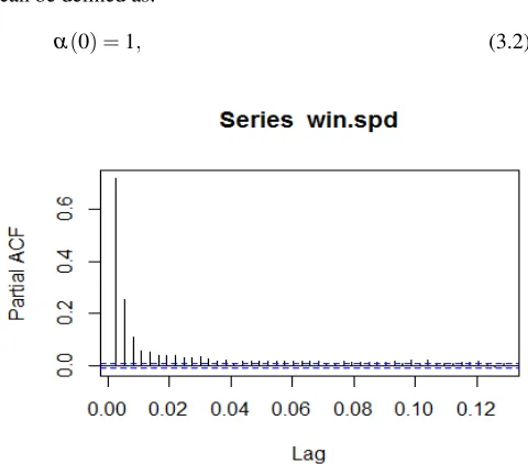
Figure 2.Autocorrelation Function for Model Identification

(4)

can be defined as:

α(0) =1, (3.2)

Figure 3.Partial Autocorrelation for Model Identification In the estimation process, errors of the model for which the computation should been calculated and assessed, along with the resulted values of the evaluated parameters. The values for the autoregressive coefficients are 0.4807 and 0.2004 and the moving average (MA) coefficient is−0.9876 for(2,1,1). The series: Wind Speed(2,1,1)model is presented as e simple models with less computation-time, in the forecasting proce-dure. In that case, a multiple seasonal model such as TBATS is required.

Figure 4.Forecasted Multiple Seasonal Model On taking in concern about seasonal decomposition, let first look on the fact that should it necessary to do that as trend component comprises under the time series, both the components that is irregular as well as seasonal. This is why decomposing the series is must require. Now for this we concluded that there is no irregularity in the shape of plot, so it is optimal not to perform seasonal decomposition for this series. The ARIMA model has some parameters which are

commonly defined as definedc,ϕ1,ϕ2, . . . ,ϕp,θ1,θ2, . . . ,θq.

Using the function auto.arimainR, this is often done by the strategy of maximum likelihood estimation assuming that time series is Gaussian. Perform auto arima on that time series data using auto.arima() function of “forecast” package. This technique helps us to finds the values of the parameters which maximize the probability of obtaining the information which we have observed previously. For models where p>0 and

q>0, the sample ACF and PACF are difficult to recognize and value in order selection thanin the special cases where

p=0 orq=0. A logical approach, however, is still available through minimization of the corrected Akaike’s information criteria (AICc) statistic [2]. AIC is known as theAkaike’s information criteria (AIC) is outlined as:

AIC=−2 ln(L) +2(p+q+k+1), (3.3)

The corrected AICc is outlined as:

AICc=AIC+2(p+q+k+1)(p+q+k+2)

(n−p−q−k−2), (3.4)

BIC (Bayesian Information Criteria) has mathematical for-mula. It should provide complexity more than AIC does:

BIC=AIC+log(T)(p+q+P−1), (3.5)

Hence, the concluding decision regarding the orderspandq

that minimize AICc must be based on maximum likelihood estimation. HereLis the likelihood of the data, andk=1 ifc6=0 andk=0 ifc=0.L, the likelihood function of the data is used to find the maximum likelihood estimates of the parameters of an ARMA process.

Table 1.Coefficients of ARIMA Model

ar1 ar2 ma1

Estimated 0.4807 0.2004 -0.9876 Std Error 0.0044 0.0044 0.0013

Σ2estimated as 3935 and log likelihood=-305418

AIC=610844.1,AICc=610844.1,BIC=610879.8. Now we do seasonal decomposition using the TBATS model. TBATS model is a time series model for series demonstrating multiple complex seasonality. The TBATS model was introduced by De Livera, Hyndman and Snyder (2011, JASA). ”TBATS” is an abbreviation denoting its salient types:

• Tfor trigonometric regressors to model multiple-seasonality

• Bfor Box-Cox transformations

• Afor ARMA errors

• T for trend • Sfor seasonality

(5)

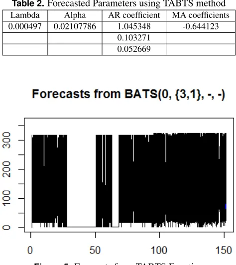
in the forecast package for R The value of the Parameters is evaluated as by using TABTS method. The value of Sigma is0.608145 and AIC is 962921.8.

Table 2.Forecasted Parameters using TABTS method Lambda Alpha AR coefficient MA coefficients 0.000497 0.02107786 1.045348 -0.644123

0.103271 0.052669

Figure 5.Forecasts from TABTS Function

Now we use decomposition procedures that are used in time series to describe the trend and seasonal factors in a time series. More wide decompositions may also include long-run cycles, day of week effects and so on. Here, we’ll only consider trend and seasonal decompositions. The main purposes for decomposition are to estimate seasonal effects that can be used to generate and current seasonally adjusted values. A seasonally adjusted value eliminates the seasonal result from a value so that trends can be seen more openly and helpful in predicting the series.

Figure 6.Result of Decomposition of Additive Series

We are aware that the regularly repeating is sessional pattern. Therefore once we arrange it seasonally we get the original time series we get:

Figure 7.Seasonal Adjusted Original Time Series

4. ETS Model

ETS i.e., Exponential Smoothing implemented by Robert G. Brown’s.

A. ETS(M,N,N): Simple exponential smoothing with multiplicative error

The models with multiplicative errors can be indicated by giving the one-step random errors defined as relative errors:

Zt=yt−yˆt/t−1, (4.1)

Hence the state space model for multiplicative form can be written as:

yt=lt−1(1+Zt)lt=lt−1(1+αZt), (4.2)

We require initial standards for those modules as well. The unknown parameters and the initial values for any exponential smoothing strategy can be surveyed by limiting the entirety of squared mistakes as in relapse investigation, yet dissimilar to the relapse case, we includes a non-straight an issue for mini-mization and henceforth we require to advance instrument to play out this. Straightforward exponential smoothing has just a single smoothing parameter and it requires just an early in-centive for the level, other exponential smoothing techniques that include a pattern or regular parts.

(6)

ahead as required [4]. Now we can evaluate the Information criteriaAIC,AICc andBICcan be used for selecting the best among 30 ETS models. The evaluated AIC is 1003202, AICc is 1003202 and BIC is 1003229.

B. Automatic Forecasting Algorithm

Automatic forecasting technique is a technique forecasting using exponential smoothingfunction in forecast package inR

[10].

The dynamically and broadly applicable for the automatic forecasting algorithm is acquired for ETS models [8], the steps followed are:

(1) For each given series, we apply all techniques that are suitable, optimizing the parameters (for both the smoothing parameters maintained and the initial state variable) of the model in each case.

(2) The best of the models can be selected according to the information criteriaAICc.

(3) Point forecast with the property of best model can be defined with optimized parameters.

(4) To obtain forecasting intervals for the best model, sys-tematic results suggested by Hyndman [9] or pretending future aspects with the illustrated paths and findingα/2 and 1−α/2 percentiles of the accurate concluded sim-ulated data at each forecasting view. In case if we used simulation, the sample paths may be created using the normal distribution for errors. The resulted Smoothing parameters are given as, the value alpha is given 0.0777, Initial states are 176.0555 and sigma is calculated as 0.729.

Figure 8.Forecasts of ETS(M,N,N)

5. Discussion and the Result Analysis

As soon as we have selected the possible models that correspond with our information, so much the ARIMA and the ETS, we realize a comparison of all of them to choose which or which are better. In our study, all data, recorded in

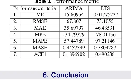
the Indian Meteorological Department, is used for the analysis in this comparison study. We collected the eight years data from 2007 to 2014, and then did the data pre-processing to clean data such as missing data and inconsistent data. The performance comparisons of ETS and ARIMA(2,1,1)model for MAE, MAPE, RMSE and ACF1 are shown below:

Table 3.Performance metric Performance criteria ARIMA ETS

1. ME 15.60954 -0.01775237

2. RMSE 67.807 73.1055

3. MAE 35.69797 46.48531

4. MPE -34.79379 -78.01136

5. MAPE 57.44789 97.21146

6. MASE 0.4457349 0.5804287

7. ACF1 0.1896902 0.490238

6. Conclusion

In this paper we have identified the comparative study of ARIMA and ETS models which match for the measurement of wind speed time-series. The model(2,1,1)exhibits the best performance. The confirmation has been done using three common quality indexes, based in correlation procedures. In this research, the performances of ARIMA and ETS are compared. ARIMA can more efficiently capture the dynamic behavior of the weather property, say, Wind Speed compared to ETS. However we could not explore all the features of ETS due to the time limitation. Therefore, the decision about the performance of ETS model is not complete and final. We need to investigate more in this direction. Our preliminary findings show that ARIMA is better than ETS.

A. Future Work

The main aim for improving the prediction performance for the time series weather prediction model is designed and developed in this work. The implemented technique is effec-tive and precise for weather prediction but some limitations of the model is also observed thus in near future need to be re-view before use of the proposed technique. The key extension of the works is the need to be increasing the training samples for collecting the training data as the performance of predic-tion is rises with the amount of informapredic-tion thus huge amount of data can solve the issues of prediction. In the future, we plan to develop our own fuzzy logic techniques for weather forecasting. Finally, we need to compare those techniques along with ARIMA model to find the best one.

Acknowledgment

(7)

References

[1] _{R. Agrawal, R.C. Jain, M.P. Jha. and Singh, Forecasting}

of ice yield using climatic variables,Indian Journal of Agricultural Science, 50 (9) (1980), 680–684.

[2] _{G.E.P. Box and G. Jenkins,}_{Time Series Analysis, The}

Forecasting and Control, Holden-Day, San Francisco, CA, 1970.

[3] _{H. Akaike, An information criterion (AIC),}_{Math Sci.,}

14(1976), 5–9.

[4] _{R.J. Hyndman and Khandakar, Automatic time series}

for forecasting: The forecast Packages for R (No. 6/07),

Monash University of Econometrics and Business Statis-tics, 2007.

[5] _{M. Tektas, Weather forecasting using ANFIS and}

ARIMA, “A case study for Istanbul. Environmental Re-search”,Engineering and Controlling, 1(51)(2010), 5–10.

[6] _{A. Agrawal, Ratnadip Adhikari and R.K. Agrawal,}_An

Introductory Study on Time Series Modeling and Fore-casting, 2007.

[7] _{M. Rahman, A.H.M. Saiful Islam, S.Y.M. Nadvi and R.M.}

Rahman, Comparative Study of ANFIS and ARIMA Model for weather forecasting in Dhaka,IEEE, 2013. [8] _{G. Jain and B. Mallick, A Review on Weather Forecasting}

Techniques, 5(12)2016.

[9] _{www.mathworks.com}

[10] _{R.H. Shumway,}_{ARIMA Models}_{, Springer Texts in}

Statis-tics, 2011.

[11] _{Shabri, Ani Samsudin, Ruhaidah, Forecasting using}

wavelet-based autoregressive integrated moving

average-models, Res, Mathematical Problems in Engineering,

Annual 2015 Issue.

[12] _{P. Srikanth, D. Rajeswara Rao and P. Vidyullatha,}

Com-parative Analysis of ANFIS, ARIMA and Polynomial Curve Fitting for Weather Forecasting,Indian Journal of Science and Technology, 2016.

[13] _{S. Singh and J. Gill, Temporal Weather Prediction using}

Back Propagation based Genetic Algorithm Technique,

International Journal of Intelligent Systems and Applica-tions (IJISA), 6(12)(2014), 55–61.

[14] _{D.K. Patrick, P.P. Edmond, T.M. Jean-Marie, Prediction}

of rainfall using autoregressive integrated moving average

model,Case of Kinshasa city (Democratic Republic of

the Congo), from the period of 1970 to 2009, 2(1) (2014), 2348–7321.

[15] _{H. Akaike, A New Look at the Statistical Model}

Identification,IEEE Transaction on Automatic Control, 19(1974), 716–723.

? ? ? ? ? ? ? ? ? ISSN(P):2319-3786

Malaya Journal of Matematik

Time-Series analysis for wind speed forecasting