Paper 12-2012-1

(UDC: 621.373.1:517.93)

The fractional distributed order oscillator. a numerical solution

J. T. Katsikadelis

Institute of Structural Analysis and Aseismic Research, School of Civil Engineering, National Technical University of Athens

Abstract

The response of one-degree-of freedom systems with fractional distributed-order (FDO) damping is studied. The dynamics of such systems constitutes the problem of the fractional distributed-order oscillator. The investigation is achieved by developing an efficient numerical method for solving FDO differential equations. The problem is treated using two approaches. In the first approach, the system of the two coupled equations governing the response of the FDO oscillator is converted into a single FDO differential equation, while in the second approach the equations are treated as a system of FDO differential equations. Numerical examples are presented for free and forced vibrations of the FDO oscillator and useful conclusions are drawn. The resonance phenomenon is also elucidated.

Keywords: fractional distributed-order differential equations; fractional distributed-order oscillator; multi-term fractional differential equations.

1. Introduction

The one degree-of freedom systems with distributed fractional order dissipation forces have been introduced recently by Atanackovic and his co-workers (Atanackovic 2002, 2003, Atanackovic et al. 2005). They result from the generalization of the multi-term fractional differential viscoelastic model by considering continuous variation of the order of fractional derivative within a closed interval. This model leads to the following initial value problem for the linear fractional distributed-order oscillator

(2)_{( ) ( )} 2 _{( ) ( )}

u t t u t g t (1)

1 1

0 ( ) 0 ( )

p p

c c

p D dp p D udp (2)

( )

1 0

( ) 1

, 1

( ) ( )

( )

( )

m t

m c

m m

u

d m m

m _t

D u t

d

u t m

dt

(3)

The initial conditions in order that the problem is well-posed should be three. Two of them are :

0 0

(0) , (0)

u u u u (4)

The third initial condition results rather from physical consideration of the deformed state at

0

t . A relation of the form 0 ku0 can be employed as the third initial condition (see

Subsection 3.2).

The system of Eqs (1), (2) is solved numerically. The solution procedure is based on the method developed by Katsikadelis for the numerical solution of distributed order fractional differential equations (Katsikadelis 2012). Numerical results for free and forced vibrations of the oscillator with ( )p ap, ( )p bp are presented. The resonance of the oscillator is also studied and interesting conclusions are drawn regarding the efficiency and accuracy of the solution method. The structure of the remaining paper is as following:

In Section 2, the first approach is described, where the two coupled equations are converted into a single FDO equation. In Section 3 the second approach is developed, where the two coupled equations are treated as a system of FDO equations, as well as the developed numerical solution. In section 4 several example problems are solved including free and forced vibrations of the FDO oscillator. Finally, Section 5 includes certain conclusions drawn from this investigation.

2. First solution approach. Conversion into a single equation

Eqs (1), (2) can be converted into a single fractional distributed order equation working as following.

Taking the Dcp derivative of Eq. (1), multiplying it with ( )p and integrating in the interval [0,1] yields

1 ₂ 1 ₂ 1 1

0 ( ) 0 ( ) 0 ( ) 0 ( ) ( )

p p p p

c c c c

p D udp p D dp p D udp p D g t dp (5)

Using Eq. (2) to replace the second integral, we obtain

1 ₂ 1 ₂ 1

0 ( ) 0[ ( ) ( )] 0 ( ) ( )

p p p

c c c

p D udp p p D udp p D g t dp (6)

which is a fractional distributed order equation of the form

1 ₂

0 { ( ) ( ) } ( )

p p

c c

p D u z p D u dp f t (7)

1 2

0

( ) ( ) ( ), ( ) ( ) cp ( )

z p p p f t p D g t dp (8)

The number of initial conditions for Eq. (6) should be ceil(2 p) 3. Eq. (6) can be solved using the numerical solution for fractional distributed-order equations developed recently by (Katsikadelis 2012). Although, this approach is straightforward, we come across here to computational difficulties, when the function g t( ) is not C1-continuous. In such a case special care is required to restore the continuity, e.g. the sigmoid function can restore the discontinuity of the step function. For this reason the second approach is recommended, since it is alleviated from this shortcoming.

3. Second solution approach. Two coupled equations.

3.1 The numerical solution

Using a quadrature rule to approximate the integral in the interval [0,1], Eq. (2) becomes a multi-term fractional differential equation (FDE). We use here the trapezoidal rule with

1 /

p K. This yields.

0 1 2 1

0 1 2 1

0

1 2 1

0

1 2 1

2 2

2 2

K K

K K

K

p p p p p

c c c K c c

K

p p p p p

c c c K c c

D D D D D

D u D u D u D u D u

(9)

where pi i p. It is p0 0 and pK 1. Hence p0

c

D and p0

c

D u u.

Next, we consider the equation

( )

c

D f q t , 0 2 (10)

Taking the Laplace transform of Eq. (10) we obtain

0 0

2

1 1 1

( ) ( )

F s f f Q s

s _{s s} (12)

where F s( ) L f t[ ( )] and Q s( ) L q t[ ( )]. The inverse Laplace transform gives

1

0 0

0

1

( ) [ 1] ( )( )

( ) t

f t f ceil f t q t (13)

Similarly, the Laplace transform of the equation

( )

c

D f q t , 0 2 (14)

is

0 ₂ 0

1 1 1

( ) ( )

F s f f Q s

s _{s s} (15)

1

1 0

0 1

[ceil( ) ceil( )] ( )( )

(2 ) ( )

t

c t

D f f q t d (16)

Apparently, Eq. (16) can be used to express the derivative D fc in terms of q t( ).

Eq. (13) is a Volterra integral equation, which is solved numerically in the interval [0, ]

t T to give q t( ) (Katsikadelis 2009). The interval [0, ]T is divided into N equal intervals t h, h T N/ (Fig. 1), in which q t( ) is assumed to vary according to a certain law, e.g. constant, linear etc. In this analysis q t( ) is assumed to be constant and equal to the mean value in each interval h. Hence, Eq. (13) at instant t nh can be approximated as

( )

f t

t 1

f 2 f

3 f 0

f fN

T nh

h h h h h h h h h h h

1 N f n

f

Fig. 1. Discretization of the interval [0, ]T into N equal intervals h T N/ .

0 0

2

1 1 1

1 ₀ 2 _{( 1)}

[ 1]

1

( ) ( ) ( )

( )

n

h h nh

m m m

n

h n h

f f ceil nhf

q nh d q nh d q nh d (17)

which after evaluation of the integrals yields

0 0

1

[ 1] n ( 1 ) ( ) m

n r

r

f f ceil nhf c n r n r q (18)

where

( )

h

c , 1( 1 ) 2

m

r r r

q q q (19a,b)

Using the same discretization for the interval [0, ]T to approximate the integral in Eq. (16), we obtain

1 0

1

[ceil( ) ceil( )] n ( 1 ) ( ) rm

c _n

r

n d f c n r n r q

D f (20)

( ) ( ) h c , 1 (2 ) h d (21a,b)

Applying Eq. (18) for f u, 2 and Eq. (20) for f u, pi (i 1,2, ,K) we obtain

0 0

1

( 1 ) ( )

n

m

n r

r

u u nhu c n r n r q (22)

1 2 2

0 1

( 1 ) ( )

i i i

i

n

p p p m

p _{i i r}

c n

r

n d u c n r n r q

D u , i 1,2, ,K (23)

where 2 2 (2) h c , 2

(2 ) (2 )

i p i i i h c p p 1 (2 ) i p i i h d p (24a,b,c)

Similarly, Applying Eq. (18) for f , 1 and Eq. (20) for f , pi ( 1,2, , 1

i K ) we obtain

0 1

ˆn ˆm

n r

r

c q (25)

1 1

1

ˆ ( 1 ) i ( ) i

i

n

p p m

p _{i r}

c _n r

c n r n r q

D , i 1,2, ,K 1 (26)

ˆ (1) h c , 1 ˆ

(1 ) (1 )

i p i i i h c

p p (27a,b,c)

After separating and decomposing the last term in the sums, Eqs (22), (23), (25) and (26) can be written as

1

2 2

0 0 1

1

( 1 ) ( )

2 2

n

m

n n r _n

r

c c

u q u nhu c n r n r q q (28a)

1

1 2 2

0 1

1

( 1 ) ( )

2 2

i i i

i

n

i p p p m i

p _{n i i r}

n c n

r

c c

q n d u c n r n r q q

D u , (28b)

1,2, , i K 1 0 ₁ 1 ˆ ˆ ˆ ˆ ˆ ˆ 2 2 n m

n n r _n

r

c c

q c q q (28c)

1

1 1

1 1

ˆ ˆ

ˆ ˆ ( 1 ) ( ) ˆ

2 2

i i

i

n

i p p i

p _{n i r}

n c n

r

c c

q c n r n r q q

Note that qn un and qˆn n. Eqs (28) constitute a set of 2K 1 equations for 2K 3 unknowns. The additional required two equations result from Eqs (1) and (9), which at t nh become

2

n n n n

q u g (29a)

1 2 1

1 2 1

0

1 2 1

0

1 2 1

ˆ 2 2 2 2 K K K K

p p p

n _{c n c n} K _{c n}

K

p p p p

n _{c n c n} K _{c n c n}

q

D D D

u _{D u D u D u D u}

(29b)

Eqs (28) and (29) are combined and written in matrix form as

n n

Ax b (30)

where it was set

2

0 0 1

1 2 1 1 2

1

1

1

0 0 0 0 1 1 0 0 0 0

0 0

2 2 2 2

1 0 0 0 0 0 0 0 0 0

2

0 1 0 0 0 1 0 0 0 0

2

0 0 0 0 0 0 0 0 0 1

2 ˆ

0 0 0 0 0 0 1 0 0 0

2

ˆ

0 0 0 0 0 0 0 0 1

2 K K K K K K c c c c c

A (31a)

1 1 1

2 2 2

1

2 2

0 0 1

1 1

1

1 2 2

1 0 1 1

1 1

2

1 2 2

2 0 2 1

1

1 2

0

0

( 1 ) ( )

2

( 1 ) ( )

2

( 1 ) ( )

2

( 1 ) (

K K n n m r n r n

p p p m

r _n

r n

p p p m

r n r n p p K K g c

u nhu c n r n r q q

c

n d u c n r n r q q

c

n d u c n r n r q q

n d u c n r n r

b 1 1 1 2 1 1 1 1 1 1 1 ₁ 1 1 1 1 1 1 ) 2 ˆ

ˆ ( 1 ) ( ) ˆ

2

ˆ

ˆ ( 1 ) ( ) ˆ

2 K K K n K p m r n r n p p r _n r n K p p

K r n

r

c

q q

c

c n r n r q q

c

c n r n r q q

, 1 2 1 1 ˆ K K n p c _n p c n p c n n _n n p c n p c n n u D u D u D u q D D q

It should be emphasized that that expressions of the matrices A and bn are presented here for the sake of understanding the solution procedure and not to be used as formulae. In programming the method, they are evaluated automatically from the relations (18) and (20) for the specified values of the parameters and , a quite simple task.

The coefficient matrix A is non singular for sufficient small h and can be solved successively for n 1,2, ,N to obtain xn. For n 1, the values q0 u0 and qˆ0

appear in Eq. (31b). These are evaluated in the following Subsection.

3.2 Evaluation of q0 u0 and qˆ0 0

For t 0, Eq. (9) gives

0 1 2 1

0 1 2 1

0

0 1 0 2 0 1 0 0

0

0 1 0 2 0 1 0 0

2 2

2 2

K K

K K

K

p p p p p

c c c K c c

K

p p p p p

c c c K c c

D D D D D

D u D u D u D u D u

(32)

The derivatives Dcpi 0 and D ucpi 0 0 pi 1 can be expressed in terms of 0 and u0 using

the relations (Katsikadelis 2009, Appendix)

1 1

0

1

(0) 2 2

(2 )

i i i

p p p

c

i

D h

p (33a)

1 1

0

1

(0) 2 2

(2 )

i i i

p p p

c

i

D u h u

p (33b)

Thus, Eq. (32) yields

1 0 2 0 1 0u 2 0u (34)

whre

0 1

2 ,

1

1 1

2 1

1

2 2

(2 ) 2

i i

K

K

p p

i i

i

h

p (35a)

0 1

2 ,

1

1 1

2 1

1

2 2

(2 ) 2

i i

K

K

p p

i i

i

h

p (35b)

An alternative relation in place of Eq. (34) could be derived, if another type of the fractional derivative would be employed. For example a relation of the form ku0 was derived in (Atanackovic 2003), when the Riemann-Liouville fractional derivative was employed. For our examples the relation

1 0 2 0u (36)

is employed as the third initial condition

2

0 0 0 0

q u g (37)

Eqs (34), (35) and (37) can be used to evaluate the not specified quantities q0 u0, qˆ0 0

and 0.

4. Numerical examples

On the basis of the previously developed numerical solution approaches two computer codes have been written in MATLAB and the free and forced vibrations of the FDO oscillator are studied. The numerical results have been obtained taking ( )p ap, ( )p bp with a and b constants. For a b, Eq. (2) becomes u and Eq. (1) yields

(2)_{( ) (} 2_{) ( ) ( )}

u t u t g t (38)

Thus, the response of the oscillator becomes undamped elastic with eigenfrequency

2 1/2

( )

el as it was reported in (Atanackovic 2003). Since there are no other numerical or analytical solutions for comparison, this fact is employed to attest the reliability and accuracy of the results. The results shown here have been obtained with the second approach and they actually are identical to those obtained using the first approach.

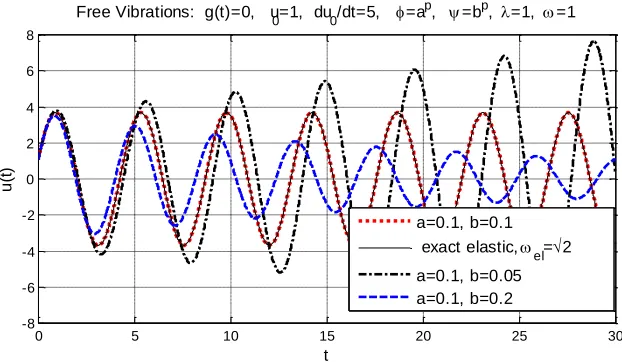
Example 1.Free vibrations

The free vibrations of the FDO oscillator are studied. The results have been obtained with

10

K and t 0.01, 1, 1. In Fig. 2, the response is shown for various values of

a and b. For a b the elastic response results, which is identical to the exact solution with

2

el . Note that for a b the amplitude increases. This was anticipated since the second law of thermodynamics is violated (Atanackovic 2003). Moreover, in Fig 3, the response of the oscillator is shown for various values of the parameter .

Fig. 2. Response of the FDO oscillator in Example 1.

0 5 10 15 20 25 30

-8 -6 -4 -2 0 2 4 6 8

t

u

(t

)

Free Vibrations: g(t)=0, u

0=1, du0/dt=5, =a

p_{, =b}p_{, =1, =1}

a=0.1, b=0.1

exact elastic, 

el=2

Fig. 3. Response of the FDO oscillator for various values of in Example 1.

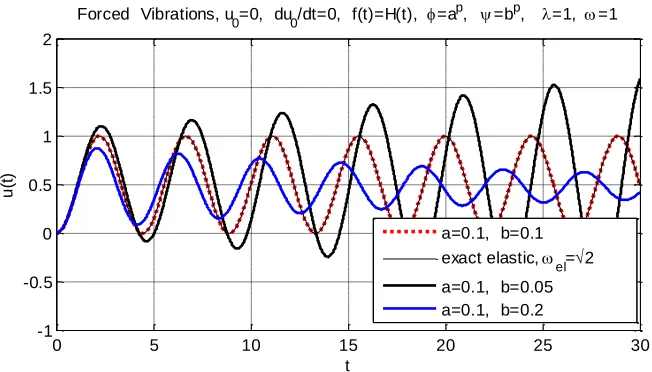
Example 2 Forced vibrations under step function

In this example the forced vibrations of the FDO subjected to the Heaviside step load function, ( ) ( )

g t H t , are studied. The response obtained with K 10, t 0.01, 1, 1 and various values of a and b is shown in Fig. 4. Note that for a b the solution is identical to the elastic with el 2.

Fig. 4. Response of the FDO oscillator in Example 2.

Example 3. Forced vibrations under harmonic excitation

In this example the forced vibrations of the FDO subjected to the harmonic excitation

0

( ) sin

g t p t are studied. The response obtained with K 10, t 0.01,

0 1 2 3 4 5 6 7 8 9 10

-1 -0.5 0 0.5 1

t

u

(t

)

Free Vibrations: g(t)=0, u

0=1, du0/dt=0, =a

p_{, =b}p_{, =1}

=1, a=0.1, b=0.1 =1,exact elastic, _el=2 =5, a=0.1, b=0.1 =5,exact elastic, _el=6 =10, a=0.1, b=0.15

0 5 10 15 20 25 30

-1 -0.5 0 0.5 1 1.5 2

t

u

(t

)

Forced Vibrations, u₀=0, du₀/dt=0, f(t)=H(t), =ap, =bp, =1, =1

a=0.1, b=0.1

exact elastic, _el=2

0

1.2 , 3,p 1, 1 and various values of a and b is shown in Fig. 6. Note that

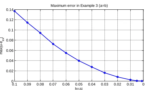
for a b the solution is identical to the elastic with 10. Finally, in Fig.6 the convergence of the maximum error max |u uex| versus the time step h t in the interval

(0 t 10) is shown.

Fig. 5. Response of the FDO oscillator in Example 3.

Fig. 6. Maximum error versus integration time step h tin Example3.

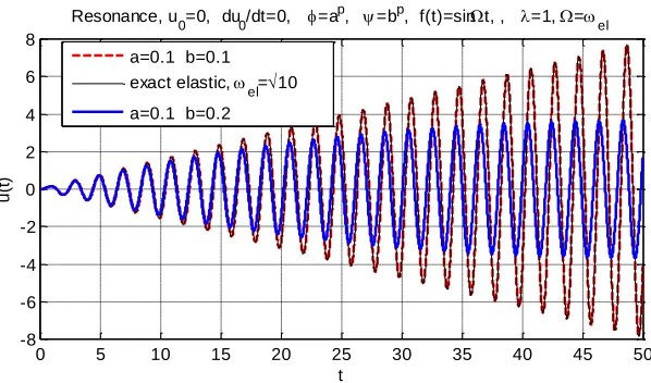
Example 4. Resonance of the FDO under harmonic excitation

In this example the resonance of the FDO under harmonic excitation g t( ) p0sin t is

studied. The response is obtained with K 10, t 0.01, 1, p0 1, 3. Fig. 7

shows the case . For a b the solution is identical to the elastic response with

0 5 10 15 20 25 30

-0.8 -0.6 -0.4 -0.2 0 0.2 0.4 0.6 0.8

t

u

(t

)

Forced Vibrations, u

0=0, du0/dt=0, =a

p_{, =b}p_{, f(t)=sint, =1.2, =3}

a=0.1 b=0.1

exact elastic, _el=10

a=0.1 b=0.2

0 0.01 0.02 0.03 0.04 0.05 0.06 0.07 0.08 0.09 0.1 0 0.02 0.04 0.06 0.08 0.1 0.12 0.14

h=t

Maximum error in Example 3 (a=b)

m

a

x

|u

-e

ex

2 1

el , which however is not in resonance. Resonance occurs in the elastic system,

when el 10. This is shown in Fig. 8.

Fig. 7. Response of the FDO oscillator in Example 4.

Fig. 8. Resonance in the elastic response, a b, el.

4. Conclusions

A numerical method has been presented for the solution of the equations governing the response of the fractional distributed order oscillator. Free and forced vibrations have been studied. The numerical results elucidate the dynamic response of the oscillator under fractional distributed order damping and validate the finding reported by other investigators that the elastic response results for ap bp. This finding has been used here to check the accuracy of the developed

0 5 10 15 20 25 30 35 40 45 50

-2 -1.5 -1 -0.5 0 0.5 1 1.5 2

t

u

(t

)

Forced Vibrations, u

0=0, du0/dt=0, =a

p_{, =b}p_{, f(t)=sint, =}

a=0.1 b=0.1

exact elastic, 

el=(1+ 2₎1/2

a=0.1 b=0.2

0 5 10 15 20 25 30 35 40 45 50

-8 -6 -4 -2 0 2 4 6 8

t

u

(t

)

Resonance, u₀=0, du₀/dt=0, =ap, =bp, f(t)=sint, , =1, =_el

a=0.1 b=0.1 exact elastic, _el=10

numerical solution. The resonance of the oscillator is also studied. The numerical results demonstrate the efficiency and accuracy of the proposed method.

Извод

Осцилатор са фракционо распоређеним редом. Нумеричко решење

Institute of Structural Analysis and Aseismic Research, School of Civil Engineering, National Technical University of Athens

Резиме

Разматрају се системи са једним степеном слободе који имају фракционо распоређен ред пригушења (FDO). Динамика оваквих система се своди на проблем осцилатора са фракционо дистрибуираним редом. Истраживање је остварено развијањем ефикасне нумеричке методе за решење (FDO) диференцијалних једначина. Проблем је разматран користећи два приступа. У првом приступу спрегнути систем основних једначина FDO осцилатора је сведен на једну FDO диференцијалну једначину, док код другог приступа једначине се разматрају као систем FDO диференцијалних једначина. Нумерички примери су дати за слободне и принудне осцилације FDO осцилатора и изнети су корисни закључци. Расветљен је такође и феномен резонанце.

Кључне речи: диференцијалне једначине са фракционо дистрибуираним редом, осцилатор са фракционо дистрибуирани редом, мултичлане фракционе диференцијалне једначине.

References

Atanackovic, T. M. (2002). A generalized model for the uniaxial isothermal deformation of a viscoelastic body, Acta Mechanica, 159, 77-86.

Atanackovic T.M. (2003), On a distributed derivative model of a viscoelastic body, C. R. Mecanique, 331.

Atanackovic T.M., Budincevic M. and Pilipovic S. (2005). On a fractional distributed-order oscillator, J. Phys. A: Math. Gen. 38 6703–6713

Katsikadelis, J. T. (2009). Numerical solution of multi-term fractional differential equations, ZAMM, Zeitschrift für Angewandte Mathematik und Mechanik, 89 (7), 593-608.