Partitional Clustering Techniques for
Multi-Spectral Image Segmentation
Danielle Nuzillard and Cosmin Lazar
CReSTIC, UFR Sciences, Moulin de la Housse, University of Reims 51687 Reims cedex 2, France. IFTS, University of Reims, 07 Bd. Jean Delautre, 08000 Charleville-M´ezi`eres, France.
Email:{danielle.nuzillard, cosmin.lazar}@univ-reims.fr
Abstract— Analyzing unknown data sets such as multi-spectral images often requires unsupervised techniques. Data clustering is a well known and widely used approach in such cases. Multi-spectral image segmentation requires pixel classification according to a similarity criterion. For this particular data, partitional clustering seems to be more appropriate. Classical K-means algorithm has important drawbacks with regard to the number and the shape of clusters. Probability density function based methods overcome these drawbacks and are investigated in this paper. Two main steps in data clustering are dimension reduction and data representation. Methods like PCA and ICA often perform dimension reduction step. To achieve a complete and more reliable representation of the data, a magnitude-shape representationis described, it takes into account both the magnitude and shape similarities between pixels vectors. The bases of PCA and magnitude-shape representationare explored to highlight the main differences and the advantages of our method over PCA. Experimental results confirm that this method is a reliable alternative to classical linear projection methods for dimension reduction.
a) Index Terms: multicomponent data, probabil-ity densprobabil-ity function, dimension reduction, partitional clustering, similarity measures, magnitude-shape rep-resentation.
I. INTRODUCTION
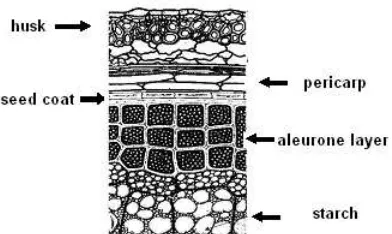
The knowledge of biological structures in plants is a very important task to valorize agronomical resources. Our work is in keeping with the identification and the repartition of various tissues in cereals. Actually cereal grains are constituted by tissues which are superimposed. The central part contains starch and the external layers serve as protection. Those contain pure natural fluorescent components : cutin, ferulic acid, lignin whose signatures recover partially. Confocal laser microspectrofluorometry enables to visualize autofluorescence of tissues. Many laser excitations associated with a set of various filters in reception allow to get pseudo multi-spectral images. In a former work, techniques of Independent Component Analysis (ICA) have been applied to isolate pseudo-spectra of pure chemical compounds and their proportion map from a multispectral image of a barley grain [1], [2]. In [3], the relationship between Blind Source Sepa-ration (BSS) methods and classification was examined through an application in teledetection. In this example, it was possible to compare both approaches because the result was known by direct land observation. Now, in the
framework of the study of the barley grain, two pixel classification methods are compared, they do not make any assumption neither on the shape of classes nor on their number.
The accuracy of a clustering method for multidimen-sional data is strongly depending on data representation. A representation in a lower dimension feature space re-quires dimension reduction techniques. The most popular algorithms for dimension reduction are linear projections such as Principal Component Analysis (PCA), Karhunen-Loeve transform (KL) or Factor Analysis (FA). ICA algorithms [4] can also be used for this purpose with mul-tiple advantages: besides the implicit dimension reduction these methods perform a more suitable transformation of the data by imposing a more general constraint: the in-dependence. Linear projection methods such as PCA and Non Negative Matrix Factorization (NNMF) [5] are tested as pre-processing methods to achieve a two-dimensional data representation.
We also propose a ”magnitude-shape representation”, where each data is defined by its magnitude (its relative distance from the origin of the working basis) and its ”shape” (its relative linear correlation with a reference vector). We must state that the linear correlation does not completely define a vector’s shape but it is a good approximation for this purpose.
A more deep insight in the bases of PCA and magnitude-shape representation will serve like argument to validate our method. It is well known that the magni-tude and the orientation offer complementary informa-tion about multi-component data. We show that PCA merges these information into a single coefficient, while the magnitude-shape representation uses magnitude and orientation independently to provide a more discriminant representation.
II. DATA PRE-PROCESSING
Cluster analysis is a tool for exploring multi-component data and it must be supplemented with techniques for visualizing data. The most direct visualization is the two-dimensional plot showing the objects to be clustered as points. A two-dimensional representation of multivariate data is not always valid but when does, it is helpful to verify the results of the clustering algorithm [6]. The principle of the linear projection methods for dimen-sion reduction of multivariate data as well as the two-dimensional magnitude-shape representation of data are presented below.
A. Dimension reduction
Dimension reduction is a common pre-processing step for clustering analysis. It consists in mapping a d -dimensional set of patterns onto a m-dimensional space, where m < d, usually m = 2. The main motivation is to allow visual inspection of multivariate data. When a reasonably accurate representation is obtained, data are clustered and results are validated [6]. The most popular dimension reduction techniques are orthogonal linear projections. A linear projection is expressed as follows:
yi=Hxi (1)
where yi is an m-dimensional column vector, xi is a d-dimensional column vector andH is anm×dmatrix. Among these, Karhunen-Loeve method and PCA are commonly used.
BSS methods are a reasonable alternative to the linear projection methods mentioned above. The orthogonality condition is replaced by the independence constraint which is more general and which may render the results meaningful. Moreover, specific applications impose phys-ical constraints. In the case of the multi-spectral images, the non-negativity of the data was already evoked in several frameworks [1], [2]. Here the NNMF [5] algorithm performs dimension reduction and the results of clustering are presented in section IV.
B. Magnitude-shape representation
In the following we consider pixels as pseudo-spectra and pseudo-spectra as vectors. The mathematical defini-tion of vectors identity states that two identical vectors have the same magnitude and the same direction; the assumption that the vector magnitude is independent of its direction is also true, meaning that the magnitude and the direction offer complementary information about vectors. Moreover, vectors are uniquely and completely defined by their magnitude and their direction (or shape). When comparing two spectra or two pixels we compare their magnitude and their direction or their shape. The most common way to compare vectors magnitude is to use the Euclidian distance as a similarity measure, which is nothing else but one instance of the Minkowski metric.
Dk= [ d
X
i=1
(Ai−Bi)k]1/k (2)
wherek²RandA, Bare two vectors.
The Euclidian distance is often cited in the literature regarding image classification and unsupervised learning, it is characterized as ”...the simplest measure of vector distance, but not an accurate one”[7]. Euclidian distance is depending on the magnitude of the square subtractive differences vector but not on its shape. It is the basic sim-ilarity measure used by Isodata and K-means clustering.
Shape information is not commonly used for multi-variate clustering because in most applications the main dissimilarities between objects depend on their magnitude not their shape. But ignoring the shape information may induce severe errors in the overall result. The shape information is justified and even of high importance ”for the situations where all variables have been measured on the same scale and the precise values taken are important only to the extent that they provide information about the object’s relative profile” [8]. Our strategy is to combine magnitude and shape information into a unique data representation.
There are several measures which test the similarity of shape between two vectors. Spectral angle is the d-dimensional extension of two-dimensional geometric angle and it is used as the spectral distance criterion for the supervised classification algorithm Spectral Angle Mapper (SAM). The spectral angle is defined as follows:
SA= arccos A TB
kAkkBk (3)
The correlation coefficient is a common statistic mea-sure of the strength of the linear relationship between two random variables. Although it does not describe completely the shape similarities between two random variables, it is commonly used for this purpose by the data analysis community. The correlation coefficient is defined as follows:
r=
Pd
i=1(Ai−µA)(Bi−µB)
(d−1)σAσB (4)
whereµA,µB,σA,σB are respectively the mean and the standard deviation of A and B.
C. Magnitude-shape representation versus PCA
The Principal Component Analysis can be expressed as:
N ewData= (eig1. . . eigm)T×(X1X2. . . Xn) (5)
where X is the data matrix and eigi is the ith eigen vector of the covariance matrix ofX.
N ewData=
eig1·X1 . . . eig1·Xn
eig2·X1 . . . eig2·Xn ..
.
eigm·X1 . . . eigm·Xn
(6)
The dot product eigi·Xk is written as:
eigi·Xk =|eigi| · |Xk| ·cos(eigi, Xk) (7)
Suppose that |eigi| = 1, then the new data is com-puted as the product between the euclidian norm of the pattern vector and its relative direction to the principal components.
Since the magnitude and data orientation offer com-plementary information, one may expect to use both of them independently to describe the data. In PCA, these information are merged into a single coefficient which is the data projection onto the principal components.
In our magnitude - shape representation, both magni-tude and orientation information are used independently to describe the data. The aim is to obtain a more discriminat-ing representation which could lead to a more reliable data grouping. Themagnitude - shape representationexpresses each pattern according to functions which intervene in the PC transform: the magnitude and the directions rela-tively to the principal components. So instead of mnew attributes, there are m+1, m attributes representing the patterns direction relatively to the principal components and another attribute representing the patterns norm.
So, the final data can be written as:
N ewData=
|X1| . . . |Xn| cos(X1, eig1) . . . cos(Xn, eig1)
.. .
cos(X1, eigm) . . . cos(Xn, eigm)
(8) The cosine between two vectors is nothing but the geometrical interpretation of the correlation coefficient between them, so the magnitude - shape representation is achieved.
N ewData=
|X1| . . . |Xn|
r(X1, eig1) . . . r(Xn, eig1) ..
.
r(X1, eigm) . . . r(Xn, eigm)
(9)
III. PARTITIONAL CLUSTERING METHODS The clustering problem has been addressed in many contexts and by researchers in many disciplines. Recent frameworks in the domain of image analysis use this tool in applications such as image segmentation by pixel grouping. Among the existing methods, the partitional clustering algorithms are the most appropriate for such applications. This section focuses on partitional cluster-ing algorithms based on the probability density function estimation.
A. Principe
In [6] the problem of partitional clustering is stated as follows: ”givennpatterns in ad- dimensional metric space, determine a partition of the patterns intoKgroups or clusters such that the patterns in a cluster are more similar to each other than patterns in different clusters”. A cluster criterion (global or local) must be adopted to. Global criteria require some prototypes to assign each pattern to a cluster but often they are not available. Then local criteria, which form clusters by means of local structure such as high-density areas or by assigning a particular pattern and its knearest neighbors to the same cluster, are the most appropriate.
B. Sch¨olkopf et al. [9] argued that ”an extreme point a view is that unsupervised learning is about estimating densities”. They also stated that ”knowledge of the density of a data set would allow us to solve whatever problem can be solved on the basis of the data”. This is why, we focus on the density based clustering methods.
There are several ways to estimate a density from a data distribution. The simplest way is to evaluate its histogram. One of the most known density estimation methods in the statistical literature is the Parzen method [10]. B. Sch¨olkopf et al. [9] proposed a method based on the support vector theory that ”computes a binary function that is supposed to capture regions in input space where the probability density lives, or its support”.
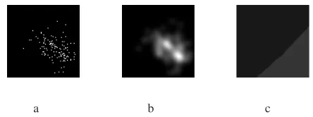
B. Parzen-Watershed Algorithm
a b c
Figure 1. Parzen-watershed on simulated data; a - the scatter-plot of two overlapped gaussian distributions represented in a discrete 64x64 feature space, this feature space is visualized as
an image; b - the estimatedpdf; c - the influence zones.
pdf p(xi)of the whole data set in the feature space. This is done according to the Parzen method [10] for which the point distribution (one object corresponds to one pointxi in feature space) is transformed into a quasi-continuous distribution p(xi) through a convolution by a smoothing kernel:
p(xi) =λ N
X
k=0
K(xi−yk
h ) (10)
where K is a smoothing kernel of size h and λ is a normalizing factor. The estimated pdf p(xi)is generally characterized by several modes, or local maxima, sepa-rated by valleys or local minima. Each mode is considered to match with a class of objects.
a b
Figure 2. SCV results on simulated data.
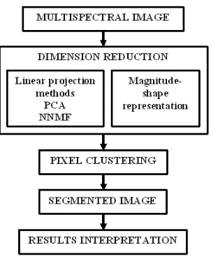
Figure 3. Scheme of the application.
Thus, the next step consists in estimating the position of the boundaries between the different classes in the feature space. Although this task is trivial for a one-dimensional feature space, it is much complicated for an n-dimensional feature space, (n >1). To split the feature space, the watershed function issued from mathematical morphology [15] or the SKIZ (SKeleton by Influence Zones) method [16] is used.
We used the SKeleton by Influence Zones procedure but the watershed method has been applied and has given similar results. This procedure consists in detecting firstly the connected components using an iterative threshold of
the estimatedpdf. The connected components are defined as one-piece subsets partitioning the whole data space. For a two-dimensional data space eight-connected neighbors are considered to define these subsets. These connected components are used as seeds to determinate the influence zones. Each point in the feature space belongs to the influence zone of that connected component which is the closest to the current point. The number of influence zones is equal to the number of connected components.
The last step consists in returning to the real image space. It is done easily because one knows where any pixel xi was mapped in the feature space, when the scatterplot was built. Thus, for any pixel of the image space, it only needs to carry back the labelcfound in the feature space, to the real space.
As for any clustering method, the question of selecting a number of classes is relevant. A stability criteria is proposed in [14] for which the number of classes is the number of modes of the estimated pdf. The number of modes itself is related to the width of the smoothing kernel h. Estimating the number of classes consists in looking at the number of modes M as a function of the parameter h. The decreasing curve M = f(h) displays some plateaus, which gives stable solutions for the number of classes.
Figure 4. Multicomponent image of a cross section of a barley grain.
C. Suport Vector Clustering (SVC)
a
b
c
d
Figure 5. First two components after linear projections: a, b - PCA; c, d - NNMF.
hyperplane when mapped back to the data space, forms a set of contours which encloses the data points. These contours are interpreted as cluster boundaries. Points enclosed by each separated contour are associated in the same cluster. As the width parameter of the Gaussian kernel decreases, the number of disconnected contours in the data space increases, leading to an increasing number of clusters [17].
Suport Vector Clustering (SVC) deals with outliers by employing a soft constant margin that allows the hyperplane in feature space not to separate all points. Large values of this parameter are suitable to deal with
a
0 5 10 15 20
0 0.2 0.4
0 5 10 15 20
0 0.5
0 5 10 15 20
0 0.2 0.4
0 5 10 15 20
0 0.2 0.4
b
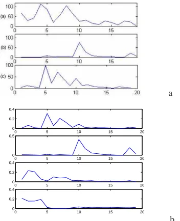
Figure 6. a - Reference spectra: cutine, ferulic acid and lignin; b - First four column vectors after the NNMF.
0 5 10 15 20
0 5 10 15 20
Kernel size
Number of classes
a
5 7 9 11 13 15 17 19 20 0
2 4 6 8 10 12 14 16 18 20
Kernel size
Number of classes
b
5 10 15 20
3 5 7 9 11 13 15 17 19 21 22
Kernel size
Number of classes
c
Figure 7. Stability of the number of classes: a - PCA representation; b - NNMF representation; c -magnitude-shape representation.
overlapping clusters [17]. To separate the data from the origin, the following quadratic equation has to be solved:
minw²F,ξ²Rlρ²R
Ã
1 2 kwk
2+1 νl
X
i
ξi−ρ
!
(11)
subject to:
w.Φ(xi)≥ρ−ξi, ξi≥0 (12)
where ρ and w are the offset and the weight vector defining the separating hyperplane andΦ(xi)is a function which maps the original data into a inner product feature space.
Since nonzero slack variables ξi, are penalized terms in the objective function, we can expect that if w andρ solve this problem, then the decision function :
f(x) =sgn(w.Φ(xi)−ρ) (13)
is positive for the most samples xi contained in the data set, whilekwkis still small. The actual trade-off between these two goals is managed by the outlier controller ν . Using multipliersαi, βi≥0 a Lagrangian is introduced:
L(w, ξ, ρ, α, β) = 1
2 kwk2+νl1
P
iξi−ρ
−Piαi((w.Φ(xi))−ρ+ξi))−
P
iβiξi (14)
and the derivatives are set to zero with respect to the primal variables w,ξ,ρyielding:
w=X i
αiΦ(xi) (15)
αi= 1
νl−βi≤
1
νl,
X
i
All samples xi for which αi > 0 are called support vectors. So the decision function f is transformed into a kernel expansion.
f(x) =sgn
à X
i
αik(xi, x)−ρ
!
(17)
Substituting equations 15 and 16 into 14 the dual problem is obtained:
min
1
2
X
ij
αiαjk(xi, xj)
(18)
subjected to:
0≤αi≤ 1
νl,
X
i
αi= 1 (19)
The valueρis recovered by exploiting that for anyαi>0 the corresponding patternxi satisfies:
ρ=w.Φ(xi) = Σiαik(xj, xi) (20)
A more detailed presentation of this method is available in [9] and [17].
Although this procedure recovers exactly the classes boundaries, for this application the SKIZ procedure [16] has been used to separate the feature space into influence zones. The binary function allows to isolate connected components in the data space that are used as seeds for the SKIZ procedure as mentioned above.
The main drawback of this method appears when it deals with overlapping clusters [11]. To render this state-ment more reliable, two overlapped gaussian distributions were simulated in a two dimensional space and a decision line is expected to separate them as well as possible. The Parzen-watershed and SVC methods were carried out and results are displayed in figures 1 and 2. By estimating the pdf at every point of the feature space, the Parzen method may reveal the slightest details in a distribution. The local maxima denote the modes in the estimatedpdf which may lead to classes separation. SVC is instead more sensitive to overlapped classes; it may offer good results when classes are well separable but it cannot reveal details which could lead to class separation; overlapped classes are either merged into a single group, either they are split in isolated groups.
IV. EXPERIMENTAL RESULTS A. Data description
A multispectral image of a cross section of a barley grain, acquired in microspectrofluorometry is analyzed to identify external tissues of the barley grain. The grains were furnished by INRA de Clermont Ferrand and the images were recorded by INRA Nantes thanks to M.-F. Devaux. The data set contains 19 images each one of 512x512 pixels. The multispectral image, presented in figure 4 is analyzed according to the general scheme presented in figure 3.
TABLE I. ENERGY DISTRIBUTION
PCA 77.4% 16.8% 2.5% 1.3% NNMF 42% 41% 12% 5%
B. Clustering results
Three dimension reduction methods have been tested as pre-processing step for pixel clustering: two linear projection methods (PCA andNNMF) and our proposal, the magnitude-shape representation. Linear projection methods realize some linear data transformations onto orthogonal or independent directions. Generally, the most part of the energy is gathered in two or three components. This allows us to perform the dimension reduction by ignoring the low energy components. The energy distribu-tion for the PCA and NNMF applied on the multispectral image under study is presented in table I. The two first resulted components after linear transformation are shown in figure 5.
One advantage of linear projection methods such ICA methods which use independence constraint to perform a linear transformation is that, besides the implicit dimen-sion reduction they perform a more realistic transforma-tion of data. By taking into account positivity constraint imposed by physical laws, the results become physically interpretable. Lignin and ferulic acid spectra are easily identified with the first two column vectors of the recov-ered matrix and are displayed in figure 6. The third and the forth lines in figure 5 correspond to a concentration map of these two fluorescent components.
The stability of the number of classes depends on the kernel size of the Parzen-watershed clustering and that dependance was studied also. Either theMagnitude-shape representationof the data or the NNMF method as a pre-processing, both reveal 5 and 4 classes with significant reliability in figure 7. Moreover the pixel classification is almost identical whatever is the pre-processing, as seen in figure 8.
SVC results in the PCA feature space are shown in figure 9. In this case, the number of classes depends on both the kernel size and the outliers controller. The solution proposed by the criteria is not as stable as that one proposed in the Parzen-watershed case.
on the aleurone layer whose principal responsible for the fluorescence properties is ferulic acid. The analysis of the data showed that ”outer and inner aleurone cell walls exhibited similar fluorescence profiles but with significantly different intensities”. Lignin and ferulic acid spectra were identified after the NNMF separation, figure 6 b, the first and the second spectra, as well as their spatial distributions are presented in figure 5 c and d. The results are similar to those presented in [18].
V. DISCUSSION ANDCONCLUSION
Clustering methods are usually composed by two main steps: a pprocessing step consisting in dimension re-duction (or feature extraction) and data representation and the second step consisting in clustering itself. Regarding the pre-processing step, linear projection methods may offer good results if the data set is described by a linear mixing model. But this is not often the case with real data sets.
We investigated an alternative to classical linear pro-jection methods: a data magnitude-shape representation which would completely define the similarities between two vectors. We can also consider this representation like a combination of the most commonly used similarity mea-sures by most clustering algorithms for multi-component image segmentation: Minkowski distance and Pearson’s correlation coefficient. It is true that the linear correlation does not completely define vector’s shape, but we used it as a good approximation as shown by the experimental results. Also it is not yet proved that the reference vector we chose can define solely the linear correlation between vectors. One way to improve the shape representation is to take into account higher order cumulants such as the symmetry or kurtosis, too.
We also make a comparative study on two partitional clustering techniques both based on the pdf estimation. The results show that estimating the entire pdf may reveal more details about the data than estimating only its support, Support Vector Clustering being incapable to distinguish between strong overlapping clusters. These details, such as peaks in the estimated pdf may lead to class separation. The Parzen method may be affected by outliers in the data set. In this case the estimated pdf has long tails and the solution of the number of classes credibility criteria may not be stable. This drawback can be overcome by considering an adaptive kernel whose size increases in low density regions of the feature space.
REFERENCES
[1] A. Elhafid, D. Nuzillard, M.-F. Devaux, N. Petrochilos, F. Belloir, ”Extraction des signatures de compos´es purs con-stituant la couche externe du grain d’orge `a partir d’images de fluorescence”, CDRom 449, Belgique, GRETSI’05, 2005.
[2] C. Gobinet, A. Elhafid, V. Vrabie, R. Huez and D. Nuzil-lard, ”About importance of positivity constraint for source separation in fluorescence spectroscopy”, CDRom 1467, Antalaya Turkey,EUSIPCO 2005.
[3] A. Bijaoui, D. Nuzillard, T. Deb Barma,”BSS, Classifica-tion and Pixel Demixing”, 5rd Int. ICA’04, pp. 96-103, Granada, Spain, 22-24 september 2004.
[4] A. Hyv¨arinen and E. Oja. Independent Component Analy-sis: Algorithms and Applications.Neural Networks, 13(4-5):411-430, 2000.
[5] D.D.Lee and H.S.Seung, ”Learning the parts of objects by non-negative matrix factorization”, Nature, 401, pp. 788-791, 1999.
[6] A. K. Jain, R.C. Dubes, ”Algorithms for Clustering Data”, Prentice Hall College Div, New Jersey March 1988.
[7] K. Fukunaga,2thedition ”Introduction to statistical pattern
recognition”,Academic Press, Inc., San Diego, 1990.
[8] B. Everitt, S. Landau, M. Leese,4thedition ”Cluster
anal-ysis”,Oxford University Press, New York, 2001.
[9] B. Sch¨olkopf, J-C. Plat, J. Shawe-Taylor, A.J. Smola, R.C. Williamson, ”Estimating the support of a high dimensional distribution”,Neural Computingvol.13, 1443–1471, 2001.
[10] E. Parzen, ” On the estimation of a probabitity density function and mode”, Annals Math. Stats. vol. 33, 1065– 1076, 1962.
[11] D. Nuzillard and C. Lazar, ”Comparison of Two Unsu-pervised Methods of Classification for Segmenting Multi-spectral Images”, International Conference on Acoustics, Speech, and Signal Processing 2006, Toulouse, France, may, 2006.
[12] J. Cutrona, N. Bonnet, M. Herbin, F. Hofer, ”Advances in the segmentation of the multi-component microanalytical images”, Ultramicroscopy, vol.103, 141–152, 2005.
[13] N. Bonnet, ”Artificial intelligence and pattern recogniza-tion techniques in microscopic image processing and anal-ysis”,Adv. Imag. Electron. Phys.vol.14, 1–77, 2000.
[14] M. Herbin, N. Bonnet, P. Vautrot, ” Number of clusterings and influence zones”,Pattern Recognition Lettersvol. 22, 1557–1568, 2001.
[15] S. Beucher, F. Meyer, ”Mathematical Morphology in Im-age Processing”,Dekker, New York, p433, 1992.
[16] J. Serra, ”Image Analysis and Mathematical Morphology”, Academic Press, New York, 1982.
[17] A. Ben-Hur, D. Horn, H. Siegelmann, V. Vapnik, ”Support vector Clustering”,Journal of Machine Learning Research vol. 2, 125–137, 2001.
[18] A. Saadi, I. Lempereur, S. Sharonov, J. C. Autran and M. Manfait, ”Spatial Distribution of Phenolic Materials in Durum Wheat Grain as Probed by Confocal Fluorescence Spectral Imaging”,Journal of Cereal Sciencevol. 28, 107– 114, 1998.
Danielle Nuzillard is currently Professor at the University of Reims Champagne Ardenne, France. She received her Ph.D. in electronics from the University of Paris XI (Orsay) France in 1986.
Her research interests include instrumentation, signal and image processing with focus on ICA methods, data clustering and pattern recognition.
a
b
c
Figure 8. Parzen-watershed clustering results: a - PCA representation : estimated pdf, influence zones and segmented image; b - NNMF representation : estimated pdf, influence zones and segmented image; c - magnitude-shape representation : estimatedpdf, influence zones and segmented image.
0 5 10 15 20 0
5 10 15 20 25 30
Kernel size
Number of classes
niu = 0.05
niu = 0.1
niu = 0.5
niu = 0.3
a
b
c
Figure 9. SVC results in the principal components feature space: a) stability of the number of classes, b) connected components and influence zones, c) segmented image.