www.atmos-meas-tech.net/7/3023/2014/ doi:10.5194/amt-7-3023-2014
© Author(s) 2014. CC Attribution 3.0 License.
Smoothing error pitfalls
T. von Clarmann
Karlsruhe Institute of Technology, Institute for Meteorology and Climate Research, Karlsruhe, Germany
Correspondence to: T. von Clarmann ([email protected])
Received: 28 January 2014 – Published in Atmos. Meas. Tech. Discuss.: 1 April 2014 Revised: 2 July 2014 – Accepted: 15 August 2014 – Published: 18 September 2014
Abstract. The difference due to the content of a priori in-formation between a constrained retrieval and the true atmo-spheric state is usually represented by a diagnostic quantity called smoothing error. In this paper it is shown that, regard-less of the usefulness of the smoothing error as a diagnostic tool in its own right, the concept of the smoothing error as a component of the retrieval error budget is questionable be-cause it is not compliant with Gaussian error propagation. The reason for this is that the smoothing error does not rep-resent the expected deviation of the retrieval from the true state but the expected deviation of the retrieval from the at-mospheric state sampled on an arbitrary grid, which is itself a smoothed representation of the true state; in other words, to characterize the full loss of information with respect to the true atmosphere, the effect of the representation of the atmo-spheric state on a finite grid also needs to be considered. The idea of a sufficiently fine sampling of this reference atmo-spheric state is problematic because atmoatmo-spheric variability occurs on all scales, implying that there is no limit beyond which the sampling is fine enough. Even the idealization of infinitesimally fine sampling of the reference state does not help, because the smoothing error is applied to quantities which are only defined in a statistical sense, which implies that a finite volume of sufficient spatial extent is needed to meaningfully discuss temperature or concentration. Smooth-ing differences, however, which play a role when measure-ments are compared, are still a useful quantity if the covari-ance matrix involved has been evaluated on the comparison grid rather than resulting from interpolation and if the averag-ing kernel matrices have been evaluated on a grid fine enough to capture all atmospheric variations that the instruments are sensitive to. This is, under the assumptions stated, because the undefined component of the smoothing error, which is the effect of smoothing implied by the finite grid on which the measurements are compared, cancels out when the difference
is calculated. If the effect of a retrieval constraint is to be di-agnosed on a grid finer than the native grid of the retrieval by means of the smoothing error, the latter must be evalu-ated directly on the fine grid, using an ensemble covariance matrix which includes all variability on the fine grid. Ideally, the averaging kernels needed should be calculated directly on the finer grid, but if the grid of the original averaging kernels allows for representation of all the structures the instrument is sensitive to, then their interpolation can be an adequate ap-proximation.
1 Introduction
The analysis of remotely sensed data of the atmosphere often leads to ill-posed or even underdetermined inverse problems. This is because the measurements do not contain enough in-formation to reconstruct the atmospheric state on a grid as fine as that chosen by the retrieval scientist. A variety of regu-larization techniques have been proposed to solve such kinds of inverse problems, among them regularization methods by Tikhonov (1963a), Twomey (1963) and Phillips (1962), as well as the maximum a posteriori scheme, which has been systematically investigated by Rodgers (2000) and which had formerly been referred to as optimal estimation (Rodgers, 1976). Any of these regularized retrievals, however, contain formal prior information.
We call prior information “formal” if it is imported via a formal constraint in the retrieval equation, as opposed to indirect prior assumptions. Indirect a priori assumptions, or indirect constraints, can be applied, for example, by simply using a finite and rather coarse grid for representation of the atmospheric state and an interpolation rule for determination of the atmospheric state between the grid points, or by re-trieving a nonlinear function of the target quantityx which constrains the result to positive (e.g. by actually retrieving the logarithm ofx) or otherwise bounded (e.g. by actually retrieving the sine or cosine ofx values). The interaction of the chosen grid and regularization is discussed, for example, in Haario et al. (2004) and references therein.
With a grid coarse enough, maximum likelihood retrievals which do not require any formal constraint or a priori infor-mation are often possible. While the effect of finite resolution is self-evident in the latter case, because nobody reasonably expects the resolution of, for example, a vertical profile be better than the grid on which it is represented, regularized retrievals lead to oversampled profiles, i.e. there are more al-titude grid points than independent pieces of information. In this case, it is essential to report the influence of the prior information on the retrieval to the user. Since the constraint can push the retrieval away from the actual true state of the atmosphere towards the prior information, the regularization causes an additional error term. This term is larger when the influence of the prior information is stronger, which is the price to pay for a reduction in the retrieval noise by regular-ization. This additional error term was initially called “null space error” (Rodgers, 1990) until it was renamed “smooth-ing error” (Rodgers, 2000).
In this paper it will be shown that this constraint diagnostic has a particular characteristic which makes the related con-cept questionable in the context of error budget. In Sect. 2 the formal environment will be presented in which the dis-cussion will take place and the notation and terminology will be clarified. In Sect. 3 the error propagation of the smoothing error will be discussed and related problems will be identi-fied. Section 4 is dedicated to the critical discussion of the attempt to save the smoothing error concept by evaluating it on a fine enough grid, and, in Sect. 5, alternative approaches to characterize the impact of prior information on the pro-file are discussed. In Sect. 6 an application will be identified for which, despite all criticism, a concept closely related to the smoothing error concept is still appropriate. Finally, in Sect. 7, the main lessons learned will be summarized and the implications on the appropriate representation of remotely sensed data will be discussed.
2 Background and notation
For formulation of a constrained retrieval we use the con-cept and notation of Rodgers (2000) with some minor ad-justments by von Clarmann et al. (2003). We minimize a
two-component cost functionc
c=(y−F (x))TS−y1(y−F (x))+(x−xa)TR(x−xa), (1)
where y is the m-dimensional vector of measurements, F the Rn→Rm signal transfer forward model, x the n -dimensional vector of the unknown components of the at-mospheric state, Sy the m×m measurement error covari-ance matrix,xa the n-dimensional a priori information on
the atmospheric state and R an n×n regularization ma-trix. This leads, after linear replacement toF (x)by xa+
K(x−xa), where K is the Jacobian matrix with elements
ki,j=∂yi/∂xj, to the following retrieval equation: ˆ
x=xa+(KTS−y1K+R)
−1KTS−1
y (y−F (xa)) (2)
=xa+G(y−F (xa)),
where theˆsymbol denotes the estimated profile, and where the so-called gain function G, which will later be used for brevity, is implicitly defined by the second line of the equa-tion. Various choices of R are possible: R=S−a1, where Sa
is the a priori covariance matrix, leads to a maximum a pos-teriori retrieval (Rodgers, 2000), while squared and scaled kth-order finite difference matrices have been suggested by Phillips (1962), Tikhonov (1963b, a) and Twomey (1963) and have systematically been investigated for remote sensing applications by, for example, Schimpf and Schreier (1997) or Steck and von Clarmann (2001). Nonlinear variants of these retrieval approaches are common but not relevant to the topic of this paper.
The dependence of the solution on the true state is charac-terized by the so-called averaging kernel matrix of dimension n×n
A=∂xˆ ∂x =(K
TS−1
y K+R)
−1(KTS−1
y K). (3) With this we can rewrite Eq. (2) as
ˆ
x=Ax+(I−A)xa, (4)
where I is then×nidentity matrix. Rodgers (1990, 2000) suggests the application of generalized Gaussian error prop-agation (cf. next section) to estimate a diagnostic quantity, which is the mapping of the expected deviation ofxa from
the actualx:
Ssmoothing=(I−A)Se(I−A)T. (5)
Se is the covariance matrix of the atmospheric state around
the mean state. The diagnostic quantity Ssmoothing is the
information. The appropriateness to include this quantity in the error budget, however, requires closer inspection. Before this, some more general caveats in the context of the smooth-ing error are summarized.
The linear estimate presented in Eq. (5) holds only if in-deedxa=<x>, where<>denotes the expectation value.
More precisely, it is required that Se represents the
covari-ance around<x>, and not the covariance aroundxaif the
latter happens not to be chosen to equal<x>, or around any other arbitrarily chosen a priori state. The use of arbitrarily chosen covariance matrices for the evaluation of the smooth-ing error is critically discussed in Rodgers (2000, p. 49), while the need to consider a possible bias between the cor-rect expectation value of the atmospheric state and the ad hoc prior chosen to constrain the retrieval is outlined, for ex-ample, in von Clarmann and Grabowski (2007). In the latter case the effect of the formal constraint is not only smoothing of the true atmospheric state, and as a consequence the so-called smoothing error has to be complemented by the addi-tional component
(I−A)(xa−<x>)(xa−<x>)T(I−A)T, (6)
which accounts for the bias ofxa.
Further, it is important that the Sematrix includes
atmo-spheric variability on all of the scales which can be repre-sented on the grid on which it is evaluated. Sematrices
con-structed from real data often happen to be singular. This can hint at a situation where the parent data do not resolve atmo-spheric variability on the small scales corresponding to the grid on which the Seis represented. In this case, Eq. (5) will
underestimate the smoothing error. The same is, of course, true if the parent data do not fully cover the true spatial and temporal atmospheric variability.
Moreover, the term “smoothing error” can be misleading, because, depending on the retrieval scheme chosen, the re-trieved profile is not necessarily a smoothed version of the true profile but can also be a combination of the a priori pro-file and the propro-file the unregularized retrieval would tend to-wards. While in many cases the profile obtained by means of Eq. (2) is smoother than the true profile, there is no reason that this should always be the case. The retrieved profile can also be shifted with respect to the true profile, or, depending on the actual prior information used, it can also have artificial structure.
Examples of error budget estimates including the smooth-ing error or with the smoothsmooth-ing error as a supplemental diagnostic quantity can be found in Worden et al. (2004), Bowman et al. (2006) and Kramarova et al. (2013).
3 Error propagation
3.1 General linear or moderately nonlinear case Let
v=f (u) (7)
for any real vectorial argumentuand any real vectorial result
v. The uncertainties ofumap onto the uncertainties ofvas
Sv≈KSuKT, (8)
where Suand Svare the error covariance matrices of vectors
uandv, respectively, and where K is the Jacobian matrix of
v=f (u)with elements∂vj∂u
i. Equation (8) is a generalization of the Gaussian error propagation law1
σvj2 ≈X i
∂v j ∂ui
2
σui2, (9)
where σui and σvj are the standard deviations represent-ing the uncertainties ofvj andui, respectively. Contrary to the latter equation, which assumes uncorrelatedui, Eq. (8) is valid also for intercorrelated errors ofui, which are ac-counted for by the related off-diagonal elements of covari-ance matrix Su. These error propagation rules are generally accepted in all cases except for grossly nonlinear functions f (u).
Application of this formalism to the mapping of measure-ment noise onto retrieved atmospheric state variables gives
Snoise≈GSyGT. (10)
3.2 Application to retrieved profiles
Typical linear operations performed with retrieved vertical profiles are transformation from one altitude grid to another, e.g. by interpolation from a coarse grid to a finer grid (cf. Rodgers, 2000, p. 162) by
ˆ
xfine=Wxˆcoarse, (11)
of which a possible inverse operation is ˆ
xcoarse=Vxˆfine=(WTW)−1WTxfine. (12)
Here,xˆcoarseandxˆfineare of dimensionsnandn˜, and W and
V aren˜×n- andn× ˜n-dimensional transformation matrices, respectively. In this context it is important to note that trans-formation from the coarse to the fine grid is reversible be-cause VW=Icoarse, i.e. back transformation from the fine to
1Although its name may suggest the contrary, this error
the coarse grid will fully restore the original coarse-grid pro-file. In contrast, transformation from the fine to the coarse grid implies an irreversible loss of information; because of WV6=Ifine, back transformation to the fine grid will not
re-store the original profile.
According to Eq. (8), retrieval noise is propagated from the coarse to the fine grid as
Snoise,fine=WSnoise,coarseWT (13)
and from the fine grid to the coarse grid as
Snoise,coarse=VSnoise,fineVT. (14)
The same equations apply to the propagation of the parame-ter error estimate. The latparame-ter is the response of the retrieval to uncertainties in the forward model parameters.
As has already been mentioned by Rodgers (2000), the en-semble covariance matrix Se cannot be transformed from a
coarser to a finer grid by means of Eq. (13), because it does not represent the variability on any scale finer than that rep-resented on its original grid. It has, however, never been dis-cussed that, as a direct consequence of this, the smoothing error as evaluated using Eq. (5) also cannot be interpolated from its native grid to any finer grid. The smoothing error of
ˆ
x represents smoothing error components only with respect to variability which can be represented on the native grid of Se.
The striking consequence of this, which has, to the best knowledge of the author, never been mentioned, is that the generalized Gaussian error propagation does not generally apply to the smoothing error. Even for linear functionsf (x), error propagation laws fail when applied to the smoothing error as soon as the linear function involves any kind of in-terpolation to any grid finer than that on which the smooth-ing error has been evaluated. Interpolation of retrieved data to grids different from (often: finer than) the initial retrieval grid are a frequent task, e.g. when databases are created in which results of different instruments are represented in a common format and on a common grid (e.g. Sofieva et al., 2013; Hegglin et al., 2013; Tegtmeier et al., 2013).
While Gaussian error propagation (Eq. 8) of the smoothing error would give
Ssmoothing,fine=WSsmoothing,coarseWT (15)
=W(Icoarse−A)Se,coarse(Icoarse−A)TWT
=(Ifine−WAcoarseV)WVSe,fine(WV)T
(Ifine−WAcoarseV)T
(cf. Rodgers, 2014, for the representation shown in the third and fourth lines of this equation), the correct linear estimate is
Ssmoothing,fine=(Ifine−Afine)Se,fine(Ifine−Afine)T, (16)
with Afine=WGcoarseKfine (Rodgers, 2000, p. 161).
Equa-tion (16) cannot be inferred via Eq. (8) from Ssmoothing,coarse.
Here, Se,fineis the ensemble covariance matrix evaluated on
the fine grid and including small-scale variability which can-not be represented on the coarse grid, Kfine is the Jacobian
which represents the sensitivities of the measurements to at-mospheric variability on the fine grid and Icoarseand Ifineare
the identity matrices on the respective grids.
The problem is caused by the fact that the smoothing er-ror does not characterize the full smoothing effect but in-stead only that part which is caused by the constraint term in Eq. (2). The additional smoothing caused by the finite grid which cannot resolve all atmospheric variability remains un-accounted for. This representation error term is assumed to be practically zero in the idealized framework by Rodgers (2000), but this assumption will be challenged in the next section.
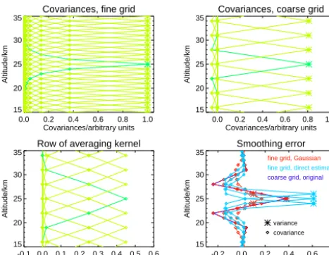
In order to demonstrate that this difference is not only of academic interest, Ssmoothing,finehas been evaluated both via
generalized Gaussian error propagation (Eq. 15) and directly on the fine grid (Eq. 16) (Fig. 1). The grid widths of the fine and the coarse grids have been chosen to be 1 and 3 km, re-spectively. For simplicity, the coarse grid was chosen to be a subset of the fine grid. The averaging kernels were assumed to be triangular in the fine grid, where the sum over the aver-aging kernel elements was unity. They were transformed into the coarse grid via
Acoarse=VAfineW (17)
(bottom left panel in Fig. 1). The ensemble covariance matrix Se,finewas constructed with diagonal values of 1 (in arbitrary
units), and exponentially decreasing all positive off-diagonal values, where the correlation length was varied from values of 1 to 20 km (upper left panel in Fig. 1). Construction of Se,coarserelies on the V matrix (upper right panel in Fig. 1).
Averaging kernels and climatological variabilities were cho-sen to be altitude-independent.
Covariances, fine grid
0.0 0.2 0.4 0.6 0.8 1.0 Covariances/arbitrary units 15
20 25 30 35
Altitude/km
Covariances, coarse grid
0.0 0.2 0.4 0.6 0.8 1.0 Covariances/arbitrary units 15
20 25 30 35
Altitude/km
Row of averaging kernel
-0.1 0.0 0.1 0.2 0.3 0.4 0.5 0.6 Averaging kernel 15
20 25 30 35
Altitude/km
Smoothing error
-0.2 0.0 0.2 0.4 0.6 0.8 Smoothing error/arbitrary units 15
20 25 30 35
Altitude/km
fine grid, Gaussian fine grid, direct estimate
coarse grid, original
variance covariance
Figure 1. Case study: the upper left panel shows the ensemble
co-variances on the fine grid (grid spacing 1 km). Only the symbols are significant – the lines are only plotted to guide the eye. The large asterisks are the variances. The variance and covariances referring to 25 km are highlighted for clarity. The top right panel shows the covariances on the coarse (grid width 3 km) grid. The lower left panel shows the averaging kernels on the coarse grid. The lower right panel shows the estimated smoothing errors (in terms of vari-ances/covariances) at 24, 25 and 26 km altitude: the smoothing er-rors on the fine grid estimated by Gaussian error estimation (red) are largest at 25 km, an altitude which coincides with an altitude of the coarse grid, and are smaller for 24 and 26 km, where the values on the fine grid depend on interpolation. The opposite is true for the direct estimates of the smoothing error on the fine grid (light blue): here the smoothing error is smallest at 25 km and larger at 24 and 26 km. More importantly, the directly estimated smoothing errors are considerably larger. This is because the relevant ensemble co-variance matrix contains larger atmospheric variability (cf. top pan-els). The original smoothing error estimate on the coarse grid (dark blue) is hardly visible because it is identical to that represented on the fine grid.
the smoothing error. The direct evaluation on the fine grid via Eq. (16) gives smoothing error variances of 0.61 (light-blue lines/symbols in the lower right panel). The smoothing errors are larger because they account for the additional variability which can be represented only on the fine grid but which is lost when smoothing errors are evaluated on the coarse grid. For larger correlation lengths in Se,fine, the smoothing
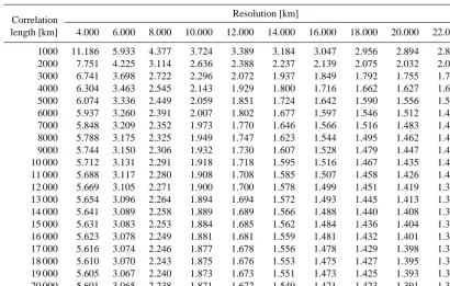
er-rors decrease but the contrast between the two ways to esti-mate it on the fine grid remains large. For a correlation length of 20 km and a vertical resolution of the retrieval of 6 km, the correctly calculated smoothing error on the fine grid is still more than 3 times larger than that estimated via Gaus-sian error propagation. For inferior altitude resolutions, this ratio becomes smaller, but even for a correlation length of 20 km and a vertical resolution of 22 km, the correctly calcu-lated smoothing error is still higher by 37 % compared to the estimate using Gaussian error propagation. Obviously, the
difference between the two ways to estimate the smoothing error does not fully disappear even if the original retrieval has been considerably oversampled (Table 1). Putting the-oretical concerns aside, dissemination of diagnostic matri-ces sampled fine enough to keep the inaccuracy implied by any further interpolation tolerably small can easily be beyond reach for reasons of the pure amount of data to be commu-nicated, and in many real applications the grid on which the diagnostic quantities are provided is defined in a way that the scales which the instrument can measure are resolved (weak gridding criterion) rather than all the scales on which atmo-spheric variability still occurs (strong gridding criterion).
Therefore either Gaussian error propagation has to be abandoned or the smoothing error problem has to be fixed in a way that the smoothing error concept becomes consistent with the generalized Gaussian error propagation law. Since Gaussian error propagation is an essential part of linear the-ory and even of quantitative empirical research in general, it might not be acceptable to drop it in favour of the cur-rent smoothing error concept. Instead, either a way needs to be determined by which the smoothing error concept can be modified such that it becomes compatible with established error propagation laws, as will be attempted in the next sec-tion, or otherwise an alternative way to report the a priori content of the retrieval which makes no use of the smoothing error concept is needed.
4 The nature of the retrieved quantities
Having understood the source of the problem and accept-ing that there exists natural variability on all physical scales (Richardson, 1920), the natural approach would appear to be to evaluate the smoothing error on an infinitesimally fine grid. This would assure that the smoothing error represents atmospheric variation on all possible scales. Of course, this ideal cannot be reached within finite-dimension algebra, but one could at least try to evaluate the smoothing error on a grid fine enough that further refinement of the grid does not im-ply additional variability. In other words, the problem should be diagnosed on a grid on which the full variability of the atmosphere can be represented (strong gridding criterion). This approach is based on the assumption that the residual smoothing error not accounted for on a finite grid converges towards zero for a grid spacing approaching zero. In the fol-lowing it will be shown that this assumption is false.
Table 1. Ratio of correctly calculated smoothing errors and smoothing errors calculated via Gaussian error propagation.
Correlation Resolution [km]
length [km] 4.000 6.000 8.000 10.000 12.000 14.000 16.000 18.000 20.000 22.000
1000 11.186 5.933 4.377 3.724 3.389 3.184 3.047 2.956 2.894 2.849
2000 7.751 4.225 3.114 2.636 2.388 2.237 2.139 2.075 2.032 2.001
3000 6.741 3.698 2.722 2.296 2.072 1.937 1.849 1.792 1.755 1.728
4000 6.304 3.463 2.545 2.143 1.929 1.800 1.716 1.662 1.627 1.603
5000 6.074 3.336 2.449 2.059 1.851 1.724 1.642 1.590 1.556 1.533
6000 5.937 3.260 2.391 2.007 1.802 1.677 1.597 1.546 1.512 1.490
7000 5.848 3.209 2.352 1.973 1.770 1.646 1.566 1.516 1.483 1.461
8000 5.788 3.175 2.325 1.949 1.747 1.623 1.544 1.495 1.462 1.440
9000 5.744 3.150 2.306 1.932 1.730 1.607 1.528 1.479 1.447 1.425
10 000 5.712 3.131 2.291 1.918 1.718 1.595 1.516 1.467 1.435 1.414
11 000 5.688 3.117 2.280 1.908 1.708 1.585 1.507 1.458 1.426 1.405
12 000 5.669 3.105 2.271 1.900 1.700 1.578 1.499 1.451 1.419 1.398
13 000 5.654 3.096 2.264 1.894 1.694 1.572 1.493 1.445 1.413 1.392
14 000 5.641 3.089 2.258 1.889 1.689 1.566 1.488 1.440 1.408 1.387
15 000 5.631 3.083 2.253 1.884 1.685 1.562 1.484 1.436 1.404 1.383
16 000 5.623 3.078 2.249 1.881 1.681 1.559 1.481 1.432 1.401 1.380
17 000 5.616 3.074 2.246 1.877 1.678 1.556 1.478 1.429 1.398 1.377
18 000 5.610 3.070 2.243 1.875 1.676 1.553 1.475 1.427 1.395 1.374
19 000 5.605 3.067 2.240 1.873 1.673 1.551 1.473 1.425 1.393 1.372
20 000 5.601 3.065 2.238 1.871 1.672 1.549 1.471 1.423 1.391 1.370
in any meaningful manner infinitesimal point on this small scale; quantities which characterize an air parcel in a statis-tical sense are not applicable any more. The characterization of the atmosphere by statistical terms implies a certain in-herent smoothing and thus the true unsmoothed state of the atmosphere is ill-defined. It is not clear with respect to which quantity the expected differences should be characterized by the smoothing error.
Admittedly, the scales discussed here are of no concern in remote sensing. However, it is not the intent here to dis-cuss the state of single molecules but simply to show that there exists no reasonable limit to which mixing ratios, num-ber densities or temperature converge for steadily decreasing scale lengths, i.e. that convergence of the smoothing error cannot safely be expected when the grid spacing approaches zero: for example, mixing of air parcels of different com-position range from planetary waves down to the molecular scale. Thus, for any finite grid, there exist sub-grid processes causing their own variability in the atmospheric state not rep-resented by Seuntil we reach the molecular scale on which
the pathological cases discussed above occur.
In conclusion, the attempt to solve the propagation prob-lem of the smoothing error by use of a grid fine enough that it is guaranteed that interpolation will never occur must be considered as failed. In more practical terms, it is fair to say that if sufficient information is available to construct Se on
a certain fine grid, then there will be scientists who are in-terested in atmospheric processes on even finer scales which have their own variability.
5 The way out of the dilemma
only an option but in fact seems to be the only reasonable choice because the concept of the ideally infinitesimally fine resolved atmospheric state has been shown to be untenable. The smoothing error concept which assumes a “true”, i.e. un-smoothed, atmosphere contradicts itself, because the evalua-tion of the smoothing error on a finite grid with its implicit smoothing through finite representation gives the notion of the retrieval characterizing a finite air volume access through the back door again; in other words it breaks with its own assumption that the “smoothing error” represents the entire smoothing component of the retrieval error relative to the “true” atmosphere in absolute, i.e. grid-independent, terms without grid-dependent representation errors.
The decision to distribute the averaging kernel matrix in-stead of the smoothing error as the main diagnostic to char-acterize the impact of the constraint of the retrieval needs further discussion. To compare the effect of the constraint to the effect of measurement errors on a grid finer than that on which the data are distributed, the user might wish to cal-culate the smoothing error on the finer grid. The user might have an Sematrix available or can construct one from known
energy cascades between scales or knowledge on relevant small-scale processes. The user can do so because Seis not
an instrument-dependent quantity, i.e. its construction does not require expert knowledge on the particular instrument. However, the user will have the averaging kernels available only on the original (coarser) grid. In this case the user would use
Ssmoothing,fine=(Ifine−WAV)Se,fine(Ifine−WAV)T, (18)
which is incorrect because WV6=Ifine. If, however, the
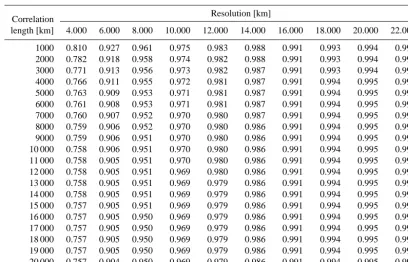
orig-inal grid had been chosen fine enough to represent all the at-mospheric variability that the instrument is sensitive to (weak gridding criterion), the error caused by the interpolation of the averaging kernel matrix can remain tolerably small. Ta-ble 2 shows the ratios of smoothing errors calculated with the correct averaging kernel matrix and those calculated accord-ing to Eq. (18) for the series of case studies from Sect. 3.2. In all cases the approximation used leads to an overestima-tion of the smoothing error, but for cases when the original coarse grid is more than 3 times finer than the resolution of the retrieval, related errors of the estimated smoothing error are smaller than 5 %. In all cases, the inaccuracy of the es-timated smoothing error due to interpolation of the averag-ing kernel is orders of magnitude smaller than inaccuracies by application of Gaussian error propagation to the coarse-grid smoothing error. Thus, it seems to be, in agreement with Rodgers (2000, Sect. 11.2.6), preferable to distribute the av-eraging kernel instead of the smoothing error.
Once having accepted the failure of the smoothing error concept as a grid-independent tool to characterize the full smoothing component of the difference between the retrieved and the true atmospheric state, it is comforting that the finite-resolution concept offers at least three further advantages:
first, the estimate of the error budget for any retrieval involv-ing a given R (which may or may not be an approximation to, or coarse sampling of, S−1
e ) no longer depends via Eq. (5)
on the choice2of the ensemble covariance matrix. Often no reliable estimate of Se is available, but any arbitrary choice
is in conflict with the smoothing error concept (cf. Rodgers, 2000, p. 48). Second, the averaging kernel is needed for a number of applications of measured data regardless, and to provide it instead of the smoothing error is advantageous for the data user. Third, error budgets of instruments whose re-trievals are performed on different grids become intercom-parable, which was not the case when the error budget still included the smoothing error. The latter is again related to the core of the problem, viz. that smoothing errors evaluated on different grids actually represent different error components. Although meaningless, it is indeed common practice to com-pare total error bars (including the smoothing component) of retrievals performed on different grids.
One implication of abandoning the smoothing error con-cept as part of the error budget is that the usual estimate of the retrieval error covariance matrix shown below is no longer valid, at least not in a general sense where transfor-mation between grids are an issue. Rodgers (1976) states that the retrieval error covariance matrix is
Sx=
KTS−y1K+S−a1
−1
. (19)
This covariance matrix which uses the a priori covariance matrix Sa as an approximation for the ensemble
covari-ance matrix Secontains both the measurement noise and the
smoothing error component (cf. Rodgers, 2000, p. 58). Thus, all caveats discussed for the smoothing error apply equally to the error estimate of Eq. (19). An error estimate free of smoothing error contributions can be made by direct appli-cation of Eq. (10) to the various error sources, viz. noise and parameter errors.
Moreover, Eq. (19) is, regardless of the discussion of the smoothing error in this paper, inapplicable to any choice of the Sa matrix except for the true climatological a priori
co-variance matrix Se. While reasonable retrievals can be
per-formed with ad hoc choices of the regularization term in Eq. (2), Eq. (19) does not provide a valid error estimate in these cases. The inadequacy of an ad hoc choice of Sewhich
has been already highlighted by Rodgers (2000, p. 48) also makes Eq. (19) inadequate for all choices of Saexcept for the
true covariance of the atmospheric state under investigation.
2Ideally, contrary to the a priori covariance matrix S
a, there is
no “choice” in the construction of Se, because it is not an ad hoc
Table 2. Ratio of correctly calculated smoothing errors and smoothing errors calculated using interpolated averaging kernels.
Correlation Resolution [km]
length [km] 4.000 6.000 8.000 10.000 12.000 14.000 16.000 18.000 20.000 22.000
1000 0.810 0.927 0.961 0.975 0.983 0.988 0.991 0.993 0.994 0.995
2000 0.782 0.918 0.958 0.974 0.982 0.988 0.991 0.993 0.994 0.995
3000 0.771 0.913 0.956 0.973 0.982 0.987 0.991 0.993 0.994 0.995
4000 0.766 0.911 0.955 0.972 0.981 0.987 0.991 0.994 0.995 0.995
5000 0.763 0.909 0.953 0.971 0.981 0.987 0.991 0.994 0.995 0.995
6000 0.761 0.908 0.953 0.971 0.981 0.987 0.991 0.994 0.995 0.996
7000 0.760 0.907 0.952 0.970 0.980 0.987 0.991 0.994 0.995 0.996
8000 0.759 0.906 0.952 0.970 0.980 0.986 0.991 0.994 0.995 0.996
9000 0.759 0.906 0.951 0.970 0.980 0.986 0.991 0.994 0.995 0.996
10 000 0.758 0.906 0.951 0.970 0.980 0.986 0.991 0.994 0.995 0.996
11 000 0.758 0.905 0.951 0.970 0.980 0.986 0.991 0.994 0.995 0.996
12 000 0.758 0.905 0.951 0.969 0.980 0.986 0.991 0.994 0.995 0.996
13 000 0.758 0.905 0.951 0.969 0.979 0.986 0.991 0.994 0.995 0.996
14 000 0.758 0.905 0.951 0.969 0.979 0.986 0.991 0.994 0.995 0.996
15 000 0.757 0.905 0.951 0.969 0.979 0.986 0.991 0.994 0.995 0.996
16 000 0.757 0.905 0.950 0.969 0.979 0.986 0.991 0.994 0.995 0.996
17 000 0.757 0.905 0.950 0.969 0.979 0.986 0.991 0.994 0.995 0.996
18 000 0.757 0.905 0.950 0.969 0.979 0.986 0.991 0.994 0.995 0.996
19 000 0.757 0.905 0.950 0.969 0.979 0.986 0.991 0.994 0.995 0.996
20 000 0.757 0.904 0.950 0.969 0.979 0.986 0.991 0.994 0.995 0.996
6 Implication for comparison of retrievals
An exception where a quantity calculated on the basis of a concept closely related to the smoothing error is still a use-ful and poweruse-ful tool is comparison of remotely sensed data according to Rodgers and Connor (2003, their Eqs. 10 to 14). These authors suggest that profiles be validated against each other by testing whether their difference, xˆ1− ˆx2, is
significant in terms of χ2 statistics. The covariance matrix of the difference, Sδ, needed for this test, however, must not include interdependent components of the smoothing error. Thus, these authors suggest that Sδbe calculated as
Sδ=(A1−A2)Sc(A1−A2)T+Sx1+Sx2, (20)
where A1, A2, Sx1 and Sx2 are the respective averaging
kernel and retrieval noise covariance matrices and where Sc is the comparison ensemble covariance matrix. The first
term on the right-hand side of this equation characterizes the smoothing difference between both these retrievals.
This estimate of the smoothing difference between two instruments’ results is necessary to judge whether the dif-ference between the retrievals is significant or whether it can be attributed to the different smoothing characteristics of the retrievals. In this context, it is not necessary to know the smoothing error relative to the true atmospheric state as it is sufficient to characterize the difference between the smoothing characteristics. Following the Rodgers and Con-nor (2003) scheme, the difference is calculated on a common so-called “intercomparison grid”, which should generally be
at least as fine as the parent grids. When the difference ˆ
x1− ˆx2between the profiles is calculated on this grid, any
degradation of the knowledge of the atmospheric state due to the representation on a finite grid is the same for both pro-files and thus cancels out, provided that Schas been evaluated
on the intercomparison grid or any grid finer than that but is not a result of interpolation, and the grid is fine enough to ensure that the averaging kernels represent all the scales that the instruments are sensitive to (weak gridding criterion) (see Appendix). This implies that, when differences of profiles are considered, the problematic component of the smoothing error, which is the difference between the true atmosphere sampled on the comparison grid and the true atmosphere at “infinite resolution”, has no relevance anymore, and theχ2 analysis is still valid.
The approach of Rodgers and Connor (2003), however, is not without pitfalls: it is essential that the a priori covariance matrix of the comparison ensemble, Sc, represents all
vari-ability of the atmospheric state on the comparison grid. For reasons discussed in Sect. 3.2, the a priori covariance matrix cannot simply be interpolated to the comparison grid.
In summary, the smoothing difference, if calculated cor-rectly, is still a useful quantity, while the parent smoothing errors of the original profiles are affected by the problems discussed in the previous sections and thus should not be part of an error budget.
then often be regarded as nearly ideal, andx in Eq. (4) can be replaced with the resolution profile to yield the high-resolution profile as the poorer resolving instrument would see it. This transformed high-resolution profile can then be directly compared to the poorly resolved profile. This ap-proach has first been proposed and demonstrated by Connor et al. (1994).
7 Conclusions
The following discussion is limited to retrievals using formal a priori information. Recommendations are conditional, as-suming that the decision in favour of a constrained retrieval has already been made. Alternatives which avoid the whole problem, such as maximum likelihood retrievals without a formal constraint (cf., for example, Carlotti, 1988), may be worthwhile trying but are beyond the scope of this discus-sion.
The conclusions are split into two parts, the first of which being theoretical and descriptive, and the second practical and thus prescriptive.
7.1 Theoretical conclusions
It has been shown in this paper that the quantity called smoothing error does not represent an estimate of the regularization-induced difference between the retrieved state and the “true” state of the atmosphere. Instead it charac-terizes the difference between the retrieved state and an ar-bitrary representation of the true state, where this arar-bitrary representation itself, being a representation on a finite dis-crete grid, has its own representation error which can be un-derstood as an implicit smoothing error. It has further been shown that this problem cannot be solved by representing the atmosphere on a “sufficiently fine” grid with zero representa-tion error, because the estimate of the atmospheric state does not converge to a useful value when the grid approaches an infinitesimally fine grid. This is because the quantities used to characterize the atmosphere in a statistical sense (mixing ratio, concentration, temperature) are not defined at infinites-imal resolution, which would require characterization of ex-tensionless points.
7.2 Practical conclusions
The problem of the smoothing error referring to a finite sam-pling of the atmospheric state could be considered purely philosophical and practically irrelevant, and the “smoothing error” could be treated as a theoretical term without direct correspondence to the empirical world (e.g. Carnap, 1966, 1974), if the consequence of this problem were not that the quantity called smoothing error does not, contrary to the other retrieval error components, comply with generalized
Gaussian error propagation. While the smoothing error is a valuable and intuitive retrieval diagnostic in its own right, the problems encountered in the context of error propagation cause major reservations against the smoothing error concept in the context of error budget and imply that the quantity cal-culated according to Eq. (5) thus should not be called an “er-ror” in terms of error propagation. While, if calculated cor-rectly, a smoothing difference of two profiles is still a use-ful quantity, the inclusion of the smoothing error in the error budget of a retrieval will cause confusion and will lead to in-adequate operations by data users. The use of the smoothing error should be restricted to applications where it can safely be excluded that anybody would propagate this quantity to finer grids. An option could be to replace the term “smooth-ing error” with another term which does not suggest applica-bility of Gaussian error propagation; for example, one could use the term “constraint diagnostic” instead.
When the quality of two data products is compared, it is important to evaluate the smoothing error on the same grid. Otherwise the retrieval evaluated on the finer grid will erro-neously appear to be more affected by the smoothing error than that evaluated on the coarser grid.
Appendix A: The approximate validity of the smoothing difference
We start from Eq. (20) but, for simplicity, ignore the noise terms which are not relevant here. We formulate Eq. (20) on a grid which is finer than the comparison grid:
Sδ,fine=(A1,fine−A2,fine)Sc,fine×(A1,fine−A2,fine)T.
(A1) For the fine-grid averaging kernels, the approximation Afine≈WAcoarseV is used: we get
Sδ,fine≈(WA1V−WA2V)Sc,fine (A2)
×(WA1V−WA2V)T.
We are interested to get this on the comparison grid:
Sδ≈V(WA1V−WA2V)Sc,fine (A3)
×(WA1V−WA2V)TVT
=(VWA1V−VWA2V)Sc,fine
×(VWA1V−VWA2V)T
=(A1V−A2V)TSc,fine(A1V−A2V)
=(A1−A2)VSc,fineVT(A1−A2)
=(A1−A2)Sc(A1−A2).
Acknowledgements. The author thanks T. Shepherd for
“inter-rupting his dogmatic slumber” related to established diagnostic tools and their justification, as well as A. Butz and G. Stiller for helpful discussions. The problem discussed in this paper popped up during the activities SPARC Data Initiative led by M. Hegglin and S. Tegtmeier and was further investigated in the context of the ESA Climate Change Initiative (Ozone CCI) under contract number 4000101683/10/I-NB. The author thanks the eight reviewers, among them B. J. Connor, L. Hoffmann, C. D. Rodgers, J. Tammi-nen and J. Worden, for an interesting and thorough discussion of the manuscript and numerous helpful comments, which have led to substantial improvements in the paper. The support by the Deutsche Forschungsgemeinschaft and the Open Access Publishing Fund of Karlsruhe Institute of Technology are acknowledged.
The service charges for this open access publication have been covered by a Research Centre of the Helmholtz Association.
Edited by: P. K. Bhartia
References
Bowman, K. W., Rodgers, C. D., Kulawik, S. S., Worden, J., Sarkissian, E., Osterman, G., Steck, T., Lou, M., Eldering, A., Shephard, M., Worden, H., Lampel, M., Clough, S., Brown, P., Rinsland, C., Gunson, M., and Beer, R.: Tropospheric Emission Spectrometer: Retrieval Method and Error Analysis, IEEE Trans. Geosci. Remote, 44, 1297–1307, 2006.
Carlotti, M.: Global–fit approach to the analysis of limb–scanning atmospheric measurements, Appl. Optics, 27, 3250–3254, 1988. Carnap, R.: Philosophical foundations of physics: An introduction to the philosophy of science, Basic books Inc., New York, 1966. Carnap, R.: An introduction to the philosophy of science, Basic
books Inc., New York, edited by: Gardner, M., 1974.
Connor, B. J., Siskind, D. E., Tsou, J. J., Parrish, A., and Remsberg, E. E.: Ground-based microwave observations of ozone in the up-per stratosphere and mesosphere, J. Geophys. Res., 99, 16757– 16770, doi:10.1029/94JD01153, 1994.
Connor, B. J., Bösch, H., Toon, G., Sen, B., Miller, C., and Crisp, D.: Orbiting Carbon Observatory: Inverse method and prospective error analysis, J. Geophys. Res., 113, D05305, doi:10.1029/2006JD008336, 2008.
Eckert, E., von Clarmann, T., Kiefer, M., Stiller, G. P., Lossow, S., Glatthor, N., Degenstein, D. A., Froidevaux, L., Godin-Beekmann, S., Leblanc, T., McDermid, S., Pastel, M., Stein-brecht, W., Swart, D. P. J., Walker, K. A., and Bernath, P. F.: Drift-corrected trends and periodic variations in MIPAS IMK/IAA ozone measurements, Atmos. Chem. Phys., 14, 2571– 2589, doi:10.5194/acp-14-2571-2014, 2014.
Haario, H., Laine, M., Lehtinen, M., Saksman, E., and Tamminen, J.: Markov chain Monte Carlo methods for high dimensional in-version in remote sensing, J. Roy. Stat. Soc. B, 66, 591–607, 2004.
Hegglin, M. I., Tegtmeier, S., Anderson, J., Froidevaux, L., Fuller, R., Funke, B., Jones, A., Lingenfelser, G., Lumpe, J., Pendlebury, D., Remsberg, E., Rozanov, A., Toohey, M., Urban, J., von Clar-mann, T., Walker, K. A., Wang, R., and Weigel, K.: SPARC Data Initiative: Comparison of water vapor climatologies from
inter-national satellite limb sounders, J. Geophys. Res. Atmos., 118, 11824–11846, doi:10.1002/jgrd.50752, 2013.
Kramarova, N. A., Bhartia, P. K., Frith, S. M., McPeters, R. D., and Stolarski, R. S.: Interpreting SBUV smoothing errors: an exam-ple using the quasi-biennial oscillation, Atmos. Meas. Tech., 6, 2089–2099, doi:10.5194/amt-6-2089-2013, 2013.
Neu, J. L., Hegglin, M. I., Tegtmeier, S., Bourassa, A., Degenstein, D., Froidevaux, L., Fuller, R., Funke, B., Gille, J., Jones, A., Rozanov, A., Toohey, M., von Clarmann, T., Walker, K. A., and Worden, J. R.: The SPARC Data Initiative: Comparison of upper troposphere/lower stratosphere ozone climatologies from limb-viewing instruments and the nadir-limb-viewing Tropospheric Emis-sion Spectrometer, J. Geophys. Res.-Atmos., 119, 6971–6990, doi:10.1002/2013JD020822, 2014.
Phillips, D.: A Technique for the numerical solution of certain in-tegral equations of first kind, J. Ass. Comput. Mat., 9, 84–97, 1962.
Richardson, L. F.: The supply of energy from and to atmospheric eddies, Proc. Roy. Soc. London A, 87, 354–373, (quoted after R. Benzi, “Lewis Fry Richardson” in: A Voyage Through Tur-bulence, edited by: Davidson, P. A., Kanedia, Y., Moffat, K., and Screenivasan, K. R., Cambridge University Press, 187–208, 2011), 1920.
Rodgers, C. D.: Retrieval of Atmospheric Temperature and Compo-sition From Remote Measurements of Thermal Radiation, Rev. Geophys. Space Phys., 14, 609–624, 1976.
Rodgers, C. D.: Characterization and error analysis of profiles re-trieved from remote sounding measurements, J. Geophys. Res., 95, 5587–5595, 1990.
Rodgers, C. D.: Inverse Methods for Atmospheric Sounding: The-ory and Practice, Vol. 2 of Series on Atmospheric, Oceanic and Planetary Physics, edited by: Taylor, F. W., World Scientific, 2000.
Rodgers, C. D.: Interactive comment on “Smoothing error pitfall” by T. von Clarmann, Atmos. Meas. Tech. Discuss., 7, C967– C972, 2014.
Rodgers, C. D. and Connor, B. J.: Intercomparison of re-mote sounding instruments, J. Geophys. Res., 108, 4116, doi:10.1029/2002JD002299, 2003.
Schimpf, B. and Schreier, F.: Robust and efficient inversion of ver-tical sounding atmospheric high-resolution spectra by means of regularization, J. Geophys. Res., 102, 16037–16055, 1997. Sofieva, V. F., Rahpoe, N., Tamminen, J., Kyrölä, E., Kalakoski,
N., Weber, M., Rozanov, A., von Savigny, C., Laeng, A., von Clarmann, T., Stiller, G., Lossow, S., Degenstein, D., Bourassa, A., Adams, C., Roth, C., Lloyd, N., Bernath, P., Hargreaves, R. J., Urban, J., Murtagh, D., Hauchecorne, A., Dalaudier, F., van Roozendael, M., Kalb, N., and Zehner, C.: Harmonized dataset of ozone profiles from satellite limb and occultation measurements, Earth Syst. Sci. Data, 5, 349–363, doi:10.5194/essd-5-349-2013, 2013.
Toon, G., Twigg, L. W., Walker, K., and Whiteman, D. N.: Vali-dation of MIPAS IMK/IAA temperature, water vapor, and ozone profiles with MOHAVE-2009 campaign measurements, Atmos. Meas. Tech., 5, 289–320, doi:10.5194/amt-5-289-2012, 2012. Tegtmeier, S., Hegglin, M. I., Anderson, J., Bourassa, A.,
Bro-hede, S., Degenstein, D., Froidevaux, L., Fuller, R., Funke, B., Gille, J., Jones, A., Krüger, Y. K. K., Kyrölä, E., Lingenfelser, G., Lumpe, J., Nardi, B., Neu, J., Pendlebury, D., Remsberg, E., Rozanov, A., Smith, L., Toohey, M., Urban, J., von Clarmann, T., Walker, K. A., and Wang, R. H. J.: SPARC Data Initiative: A comparison of ozone climatologies from international satel-lite limb sounders, J. Geophys. Res.-Atmos., 118, 12229–12247, doi:10.1002/2013JD019877, 2013.
Tikhonov, A.: On the solution of incorrectly stated problems and method of regularization, Dokl. Akad. Nauk. SSSR, 151, 501– 504, 1963a.
Tikhonov, A.: On the regularization of incorrectly stated problems, Dokl. Akad. Nauk. SSSR, 153, 49–52, 1963b.
Twomey, S.: On the Numerical Solution of Fredholm Integral Equa-tions of the First Kind by the Inversion of the Linear System Pro-duced by Quadrature, J. ACM, 10, 97–101, 1963.
von Clarmann, T. and Grabowski, U.: Elimination of hidden a priori information from remotely sensed profile data, Atmos. Chem. Phys., 7, 397–408, doi:10.5194/acp-7-397-2007, 2007.
von Clarmann, T., Glatthor, N., Grabowski, U., Höpfner, M., Kell-mann, S., Kiefer, M., Linden, A., Mengistu Tsidu, G., Milz, M., Steck, T., Stiller, G. P., Wang, D. Y., Fischer, H., Funke, B., Gil-López, S., and López-Puertas, M.: Retrieval of temper-ature and tangent altitude pointing from limb emission spectra recorded from space by the Michelson Interferometer for Passive Atmospheric Sounding (MIPAS), J. Geophys. Res., 108, 4736, doi:10.1029/2003JD003602, 2003.
Worden, J., Kulawik, S. S., Shephard, M. W., Clough, S. A., Worden, H., Bowman, K., and Goldman, A.: Predicted er-rors of tropospheric emission spectrometer nadir retrievals from spectral window selection, J. Geophys. Res., 109, D09308, doi:10.1029/2004JD004522, 2004.
Worden, J., Wecht, K., Frankenberg, C., Alvarado, M., Bowman, K., Kort, E., Kulawik, S., Lee, M., Payne, V., and Worden,
H.: CH4 and CO distributions over tropical fires during