Nonlin. Processes Geophys., 20, 11–18, 2013 www.nonlin-processes-geophys.net/20/11/2013/ doi:10.5194/npg-20-11-2013
© Author(s) 2013. CC Attribution 3.0 License.
Nonlinear Processes
in Geophysics
Deterministic dynamics of the magnetosphere: results of the 0–1 test
S. Prabin Devi1, S. B. Singh1, and A. Surjalal Sharma2,3
1Department of Physics, Manipur University, Canchipur, Imphal – 795003, India
2Department of Astronomy, University of Maryland, College Park, MD 20742-2421, USA
3Research Institute of Science and Technology, D.M. College of Science Complex, Imphal – 795001, India
Correspondence to: S. B. Singh ([email protected])
Received: 1 June 2012 – Revised: 4 December 2012 – Accepted: 10 December 2012 – Published: 7 January 2013
Abstract. A test for deterministic dynamics in a time series data, namely the 0–1 test (Gottawald and Melbourne, 2004, 2005), is used to study the magnetospheric dynamics. The data, corresponding to the same time period, of the auroral electrojet index AL and the magnetic field componentBz of the solar wind magnetic field measured at 1 AU are used to compute the parameterK, which is zero for non-chaotic and unity for chaotic systems. For the magnetosphere and also for the turbulent solar wind,Khas values corresponding to a nonlinear dynamical system with chaotic behaviour. This result is consistent with the Lyapunov exponents computed from the same time series data.
1 Introduction
The coupled solar wind–magnetosphere system is a highly variable dynamical system with continuous exchanges of mass, momentum and energy through many plasma pro-cesses, including magnetic reconnection (Vasyliunas, 1975). As a consequence of the continuous solar wind driving, the magnetospheric dynamics is far from equilibrium and has been described as a nonlinear system that exhibits com-plex and irregular behaviour (Sharma, 1995; Klimas et al., 1996). The complexity of the magnetosphere has been ex-tensively studied using different approaches. The first stud-ies were based on the autonomous behaviour of the magne-tosphere and thus used the data of the magnemagne-tosphere alone (Vassiliadis et al., 1990, 1991; Shan et al., 1991; Price and Prichard, 1993; Sharma et al., 1993; Sharma, 1995), and emphasized its low-dimensional behaviour. Recognizing the driven nature of the magnetosphere, the next stage of studies considered the solar wind and magnetosphere as an input– output system (Price et al., 1994; Vassiliadis et al., 1995;
Valdivia et al., 1996; Chen and Sharma, 2006). Such models capture the dynamics of magnetosphere, especially during magnetic storms and substorms. The magnetospheric sub-storm is a process in which energy stored in the magne-totail through solar wind–magnetosphere interaction is re-leased explosively, causing dramatic phenomena in various regions of the magnetosphere and ionosphere. This coupling is strongly enhanced when the interplanetary magnetic field turns southward (Akasofu, 1981). A typical substorm, with a time scale of an hour, consists of three phases, viz.: en-ergy storage in the magnetotail (growth phase), sudden un-loading or release of the stored energy (expansion phase), and a return toward the quasi-equilibrium state (recovery phase). Among the geomagnetic indices representing mag-netospheric phenomena, the auroral electrojet indices AU,
AL, and AE (Mayaud, 1980), derived from the magnetic field
variations in the high-latitude auroral zone, closely reflect the features of magnetospheric substorms. During periods of en-hanced geomagnetic activity the westward electrojet, mon-itored by the AL index, increases abruptly due to currents driven by plasma processes in the magnetotail. On the other hand, the eastward electrojet, which is monitored by the AU index, increases due to processes such as the partial ring cur-rent closure via the ionosphere in the evening sector (Feld-stein et al., 2006). Therefore, the analysis of the AL and AU indices can yield insights into the dynamics of different as-pects of the magnetosphere. The AL index reflects the vari-ability of the magnetospheric substorms and is widely used in the studies of the dynamical behaviour, as in this paper. On the longer time scales, typically 10 h, the magnetic storms are the dominant phenomenon and the storm-time substorms are most intense (Sharma et al., 2003).
natural systems, such as the Earth’s magnetosphere. The techniques of phase-space reconstruction (Abarbanel et al., 1993; Kantz and Schrieber, 1997) yield the dynamical fea-tures, such as low dimensionality and characteristic time scales, inherent in the observational time series data. A key feature of this approach is its ability to yield these domi-nant dynamical properties inherent in the data, independent of modelling assumptions. This has stimulated many applica-tions to the time series data of natural and anthropogenic sys-tems, and has provided an improved understanding of the un-derlying dynamics. During the last two decades, the nonlin-ear time series methods have been used to study the magneto-sphere using AE and AL index time series, and these studies have shown evidence of chaotic behaviour in the magneto-spheric dynamics. The first study (Vassiliadis et al., 1990) used the auroral electrojet index AE for the reconstruction of phase space and found good evidence in support of the low dimensionality of the magnetospheric dynamics. This was followed by a large number of studies using improved phase-space reconstruction techniques such as the singular spec-trum analysis (Sharma et al., 1993; Pavlos et al., 1994). The scaling properties of the magnetosphere have also been stud-ied, for example, in the form of multifractal analysis, self or-ganized criticality and intermittency (Consolini et al., 1996; Chang, 1999; Klimas et al., 2000; Freeman et al., 2000; Sit-nov et al., 2000, 2001). The low dimensionality of the mag-netospheric dynamics is mainly a geometrical property and enables the modelling of the dynamics using a small number of variables. On the other hand the Lyapunov exponents are directly related to the divergence of the neighbouring trajec-tories and thus to the chaotic behaviour. The computations of these exponents from the time series data of the magne-tosphere (Vassiliadis et al., 1991; Pavlos et al., 1999) yield at least one positive Lyapunov exponent, thus showing the presence of chaos.
The low dimensionality and chaotic behaviour derived from reconstruction of phase space from time series data using time delay embedding (Abarbanel et al., 1993; Kantz and Schrieber, 1997) are subject to uncertainties, due mainly to the limitations on the data and multiscale phenomena (Ukhorskiy et al., 2004), in yielding clear dynamical trajec-tories. In the studies using the auroral electrojet indices, the phase space reconstructed from the data and its surrogates were found to be similar (Price and Prichard, 1993; Price et al., 1994). Similarly, the computation of the Lyapunov expo-nent is subject to uncertainties. Although the improvements in the phase-space reconstruction, such as orthonormality ob-tained by using singular vectors (Sharma et al., 1993), have led to better results, it is important to use independent tech-niques for a better understanding of the magnetospheric dy-namics. In this paper, the 0–1 test for chaos (Gottawald and Melbourne, 2004, 2005) is used to study the deterministic, chaotic behaviour of magnetospheric substorms using cor-related data of the solar wind–magnetosphere system. For the magnetosphere the AL index data for the years 2001 and
2007, which correspond to the peak periods of the last solar maximum and minimum, respectively, are used. This choice of the periods of extrema in solar activity provides, in ad-dition to the study of the deterministic features, a means to study the differences in general. Since the storms and sub-storms are responses of the magnetosphere to the solar wind driver, the north–south z component of the interplanetary magnetic field (IMF), responsible for magnetic reconnection at the magnetopause, is used as a variable representing the solar wind. The analysis based on the 0–1 test is thus carried out on the IMFBz, measured at 1 AU, and AL, during the same periods. So far the 0–1 test for chaos has been applied to simulated data such as those generated from the integra-tion of Lorenz equaintegra-tions and from laboratory experiments (Falconer et al., 2007; Chowdhury et al., 2012). This paper presents the first application of the 0–1 test to the observa-tional data of a natural system. In order to validate the results obtained by this test, the Lyapunov exponents are computed using the standard techniques (Hegger et al., 1999) and the consistency among the results analyzed.
The paper is organized as follows: The next section is a brief description of the 0–1 test algorithm used in the analy-sis of the magnetospheric data. In Sect. 3 the correlated solar wind and magnetospheric data and the analysis of the dy-namical behaviour using the 0–1 test, as well as comparison with results obtained from the computation of Lyapunov ex-ponents, are presented. The main results and their implica-tions are summarized in the concluding Sect. 4.
2 Test for deterministic dynamics in time series data
The ubiquity of complex or irregular behaviour in time series data of many natural and anthropogenic systems has stimu-lated the development of techniques to characterize the in-herent dynamical features. The most widely used techniques are the different forms of phase-space reconstruction using the time delay embedding (Abarbanel et al., 1993). Implicit in this approach are the reconstructed trajectories, and many studies have been developed to improve the reconstruction (Kaplan and Glass, 1992; Kennel et al., 1992; Wayland et al., 1993). However, in many cases the dynamical features, such as trajectories, are not obtained clearly and this limits the ability of the techniques to yield conclusive results.
The 0–1 test (Gottawald and Melbourne, 2004, 2005) for characterizing the origins of the irregularity of a time series overcomes this limitation and thus provides an effective and independent technique. This test is based on two main com-ponents. In the first given time series data are used to drive the dynamics on a well-chosen group extension. The second is a theorem (Nicol et al., 2001) that states that the dynam-ics on the group extension is bounded if the underlying dy-namics is non-chaotic, but is unbounded and sub-linear if the dynamics is chaotic. The time series is used to compute a pa-rameterK, which can have values in the range 0≤K≤1,
S. Prabin Devi et al.: Deterministic dynamics of the magnetosphere: the 0–1 test 13
with the value of zero for non-chaotic and unity for chaotic systems.
This method has many advantages over the methods of computing the largest Lyapunov exponents as signatures of chaos underlying complex time series data, arising mainly from the property that it circumvents the need for phase-space reconstruction. Moreover the form, nature and dimen-sion of the underlying dynamics are irrelevant for the test; i.e. they do not pose practical limitations on the method as is the case for traditional methods involving phase-space re-construction. This method applies equally well to continuous time or discrete time systems, to experimental or computed data, and to data from ordinary or partial differential equa-tions. The test is robust, in specific cases, to contamination by noise; that is, it can cope with the presence of signif-icant amount of noise in the data. All that is required are time series data of an observation of the dynamics sampled at regular intervals; almost any reasonable function of the state of the system can be used. This makes the 0–1 test an especially easy test to implement. The test determines if a variable (to be defined later asp(tα)), derived from the time series data, corresponds to Brownian motion. This test has been applied successfully to many known deterministic sys-tems and showed near-perfect correlation between this test and the standard methods of computing Lyapunov exponents. For example, this test has been applied to the well-known Henon–Heiles and Lorenz systems, and found to be useful as a marker of the transition from regularity to chaos (Barrow and Levin, 2003). The application to the time series data from laboratory experiments has shown its utility as an analysis tool (Falconer et al., 2007; Chowdhury et al., 2012). These results support the claim (Gottawald and Melbourne, 2004) that the dimension of the dynamical system and the nature of the underlying equations are not directly relevant, since the 0–1 test does not require the phase-space reconstruction of conventional nonlinear time series methods (Abarbanel et al., 1993; Hegger et al., 1999). Sun et al. (2010) illustrated the selection of parameters of this algorithm by numerical experiments and also validated the reliability and the univer-sality of the test algorithm, by applying to typical nonlinear dynamical systems, including fractional-order dynamic sys-tem.
The 0–1 test can be implemented readily for a given datum
φ (tα)at timetα (α=1,2,3,· · ·N) with a fixed interval and representing the underlying dynamics. Choosing a random constantcR, a real number (0.7 in this study), a function p(tα), is defined as
p(tα)= α X
j=1
φ (tj)cos(j c). (1)
To characterize the growth of the function defined in Eq. (1), the test uses the mean square displacements. For Brownian motion, the average of [p(tj+α)−p(tα)] is ex-pected to grow as√tα forα=1,2,3, ...., N.Therefore, the
square of[p(tj+α)−p(tα)]should asymptotically approach linear growth with tα for sufficiently largeN. For a finite length of data, the mean square displacement is defined as
M(tα)= lim N→∞
1
N−α N−α
X
j=1
[p(tj+α)−p(tα)]2. (2)
This definition of mean square displacement requires 1αN, which implies thatM(tα)grows linearly in time ifαis in the range 1αN; practically best results are obtained when α6N/10. This test is based on the recog-nition thatM(tα) is bounded in time for regular dynamics while scaling linearly with time for chaotic dynamical fea-tures. Thus the scaling behaviour of M(tα)is the essential element for the test, and is computed from its asymptotic growth rateKdefined as
K= lim α→∞
log(M(tα)) log(tα)
. (3)
In the computations log(M(tα)+1)is used to avoid nega-tive logarithms. For a time series of finite length,Kis com-puted by performing a least square fit of log(M(tα+1)) ver-sus log(tα), in the range 16α6N/10. The processes and the underlying complexity are then characterized as non-chaotic forK'0 and chaotic ifK'1. In practice the com-puted values ofK for most time series data are expected to lie between these two limits.
The application of this test to well-known systems has demonstrated the validity of this technique. For the eight-dimensional Lorenz system (Lorenz, 1996),Khas values in the range 0.7–0.8 (Gottawald and Melbourne, 2005). Consid-ering that the Lorenz system is clearly chaotic, this indicates that the cases of actual systems, which are chaotic theK val-ues, are likely to be smaller due to the presence of noise and non-chaotic features.
3 Deterministic dynamics of the coupled solar wind–magnetosphere system
The magnetospheric conditions vary widely depending on the intensity of the solar wind driver, and its dynamical char-acteristics may reflect this dependency, at least partly. In gen-eral, the two limits in the range of activities are expected to correspond to the solar maximum and minimum. Keeping this in mind the years 2001 and 2007, which correspond to the last solar maximum and minimum, respectively, are cho-sen for this study. Among the various databases of the plasma and field variables of the magnetosphere, the auroral electro-jet indices have been used extensively in the study of its dy-namical behaviour. The index AL reflects the magnetospheric variability; considering substorm time scales of∼1 h, the 5-min averaged data are used.
Fig. 1.The componentBzof IMF and auroral electrojet indexAL
for the years 2001 (panels (a) and (b)) and 2007 (panels (c) and (d)). The dashed vertical lines mark the three-month periods or quarters.
magnetosphere. The coupling of the solar wind to the mag-netosphere is enhanced during periods when the interplane-tart magnetic field (IMF) is mainly southward and thus the z-componentBzis considered the primary driver of magne-tospheric activity. The 5 min averaged IMFBzdata at 1AU (ACE data) during the same periods as theALtime series are used for the analysis. The aim is to identify if the nonlinear chaotic behaviour of the magnetosphere is indeed inherent in its dynamics or is a direct response to the solar wind driver. TheALandBzused in this study have been obtained from the OMNI database (Combined 1AUIP Data; Magnetic and Solar Indices; http://spdf.gsfc.nasa.gov).
The IMFBz andAL index are shown in Fig. 1 for the two years 2001 (panels (a) and (b)) and 2007 (panels (c) and (d)). For each year the data are divided into four quarters (marked by the dashed vertical lines). The difference in the activity levels in these two cases are evident in both the IMF and magnetospheric data (note the different scales for the two years). TheALvariations for the intense geomagnetic sub-storms have very high values, reaching close to3000nT in a few cases during 2001. During 2007, the quiet period near the last solar minimum, the peakALvalues are reduced by a factor close to two. It should however be noted that the anal-ysis presented in this paper focuses on the overall behaviour of the dynamical system in these two periods.
For each of the data segments the values ofK are com-puted using Eqs. (1) - (3). Although the length of each time series data should be very large, there are practical consid-erations that limit the data size used in the computations. As the algorithm involves computational loops, larger data
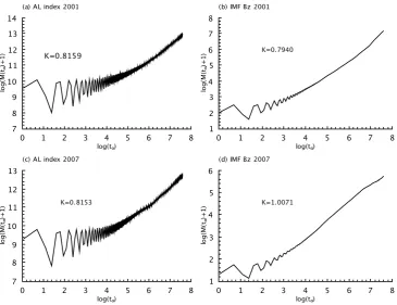
sequences lead tolonger loops and the execution time in-creases significantly, thereby decreasing the efficiency of the implementation significantly. Taking all of the above into consideration, an approximate value of the sequence length N should be selected so that the data explores enough re-gions of the attractor. The greater theNis, the closer to ideal value ofK. The plots ofK as a function of the time series lengthNare shown in Fig. 2. It is seen that in all the cases the values ofK initially show a linear increase withN and converges to finite values for largeN. Many runs of the algo-rithm were carried out for data sequences of variable lengths and it was observed that values ofKare reasonably constant forN≥15000. This clearly indicates that proper coverage of the state space occurs forN≥15000. Fig. 3 shows the plot logM(tα)vs.log(tα)for the third quarters of 2001 and 2007 for theALindices and IMFBzcalculated with 20,000 points and the corresponding K values are shown. These values, close to unity, clearly indicate the presence of chaotic be-haviour in the time series data. Similar analyses were carried out for all the data segments corresponding to the 3-month periods of the years 2001 and 2007. The computed values of K with N= 20,000 for all the cases are shown in Ta-ble 1. Also shown in this taTa-ble are the values of the largest Lyapunov exponent (LE) for these periods, and are discussed below.
The existence of a positive Lyapunov exponent is an in-dicator that determines the chaotic nature of the dynamics. Vassiliadis et al. (1991) calculated the Lyapunov exponents for theAL time series and obtained positive values in the range of0.06−0.17min−1, which clearly indicated the pres-ence of chaotic behaviour in theALtime series. In this anal-ysis of theALtime series using the 0-1 test, we have ob-tained the values of theKparameter all approximately close to 1, indicating the presence of chaotic behavior. Thus, the results of analysis using the 0-1 test are in good agreement with the earlier results (Vassiliadis et al., 1991). For a more direct comparison the Lyapunov exponents are computed for the data segments shown in Fig 2. using the TISEAN pack-age (Hegger et al., 1999). Here the time series data is rep-resented as a trajectory in an embedded space and the Lya-punov exponents are calculated by searching for all neigh-bors within a neighborhood of the reference trajectory as a function of time. We have embedded the time series data in 4 dimensions and used a delay of 6 for the purpose of com-puting the largest Lyapunov exponents. The Lyapunov expo-nents, shown in Table 1, agree well with the results of the 0-1 test for the presence of chaos, and the values agree with the earlier values (Vassiliadis et al., 1991).
TheK values shown in Fig. 2 and Table 1, have similar values for the solar minimum (2001) and maximum (2007). This however does not mean that the level of magnetospheric dynamics during these periods of very different driving by the solar wind are similar. The 0-1 test provides a characteri-zation of the inherent nature of the dynamics, viz. regular or chaotic, but does not quantify the differences in the details. Fig. 1. The componentBzof IMF and auroral electrojet index AL
for the years 2001 (a and b) and 2007 (c and d). The dashed vertical lines mark the three-month periods or quarters.
magnetosphere. The coupling of the solar wind to the mag-netosphere is enhanced during periods when the interplane-tary magnetic field (IMF) is mainly southward, and thus the
z-componentBz is considered the primary driver of magne-tospheric activity. The 5-min averaged IMFBz data at 1 AU (ACE data) during the same periods as the AL time series are used for the analysis. The aim is to identify if the nonlinear chaotic behaviour of the magnetosphere is indeed inherent in its dynamics or is a direct response to the solar wind driver. The AL andBz used in this study have been obtained from the OMNI database (Combined 1 AU IP Data; Magnetic and Solar Indices; http://spdf.gsfc.nasa.gov).
The IMF Bz and AL index are shown in Fig. 1 for the two years 2001 (panels a and b) and 2007 (panels c and d). For each year the data are divided into four quarters (marked by the dashed vertical lines). The differences in the activity levels in these two cases are evident in both the IMF and magnetospheric data (note the different scales for the two years). The AL variations for the intense geomagnetic sub-storms have very high values, reaching close to 3000 nT in a few cases during 2001. During 2007, the quiet period near the last solar minimum, the peak AL values are reduced by a factor close to two. It should however be noted that the anal-ysis presented in this paper focuses on the overall behaviour of the dynamical system in these two periods.
For each of the data segments, the values ofKare com-puted using Eqs. (1)–(3). Although the length of each time series data should be very large, there are practical consid-erations that limit the data size used in the computations. As the algorithm involves computational loops, larger data se-quences lead to longer loops and the execution time increases
Table 1. TheKvalues of the 0–1 test for chaos and the correspond-ing Lyapunov exponents, computed uscorrespond-ing the Hegger et al. (1999) algorithm, for the 3-month epochs of 2001 and 2007.
Year Epoch Time series K K LE LE
lengthN (AL) (Bz) (AL) (Bz)
2001 Jan–Mar 0.7596 1.0949 0.1313 0.1110 Apr–Jun 0.8320 0.8101 0.1255 0.1052 Jul–Sep 0.8159 0.7940 0.1219 0.0983 Oct–Dec 20 000 0.7558 0.9844 0.1227 0.0855
2007 Jan–Mar 0.8335 0.9171 0.1016 0.0914 Apr–Jun 0.9352 0.9760 0.1080 0.1027 Jul–Sep 0.8153 1.0071 0.1063 0.0986 Oct–Dec 0.7752 0.6946 0.0964 0.0905
significantly, thereby decreasing the efficiency of the imple-mentation significantly. Taking all of the above into consider-ation, an approximate value of the sequence lengthNshould be selected so that the data explore enough regions of the attractor. The greater the N is, the closer to ideal value of
K. The plots of K as a function of the time series length
N are shown in Fig. 2. It is seen that in all the cases the values ofKinitially show a linear increase withNand con-verge to finite values for largeN. Many runs of the algo-rithm were carried out for data sequences of variable lengths, and it was observed that values ofKare reasonably constant forN≥15 000. This clearly indicates that proper coverage of the state space occurs for N≥15 000. Figure 3 shows the plot logM(tα)vs. log(tα)for the third quarters of 2001 and 2007 for the AL indices and IMF Bz calculated with 20 000 points, and the correspondingK values are shown. These values, close to unity, clearly indicate the presence of chaotic behaviour in the time series data. Similar analy-ses were carried out for all the data segments correspond-ing to the 3-month periods of the years 2001 and 2007. The computed values ofKwithN=20 000 for all the cases are shown in Table 1. Also shown in this table are the values of the largest Lyapunov exponent (LE) for these periods, and are discussed below.
The existence of a positive Lyapunov exponent is an indi-cator that determines the chaotic nature of the dynamics. Vas-siliadis et al. (1991) calculated the Lyapunov exponents for the AL time series and obtained positive values in the range of 0.06–0.17 min−1, which clearly indicated the presence of chaotic behaviour in the AL time series. In this analysis of the
AL time series using the 0–1 test, we have obtained the values
of theK parameter all approximately close to 1, indicating the presence of chaotic behaviour. Thus, the results of anal-ysis using the 0–1 test are in good agreement with the ear-lier results (Vassiliadis et al., 1991). For a more direct com-parison, the Lyapunov exponents are computed for the data segments shown in Fig. 2 using the TISEAN package (Heg-ger et al., 1999). Here the time series data are represented as a trajectory in an embedded space and the Lyapunov expo-nents are calculated by searching for all neighbours within
S. Prabin Devi et al.: Deterministic dynamics of the magnetosphere: the 0–1 test 15 K 0 0.2 0.4 0.6 0.8 1 1.2
Time series length N
0 5,000 10,000 15,000 20,000 25,000 Jan--Mar Apr--Jun Jul--Sep Oct--Dec (b) IMF Bz 2001
K 0 0.2 0.4 0.6 0.8 1
Time series length N
0 5,000 10,000 15,000 20,000 25,000 Jan--Mar Apr--Jun Jul--Sep Oct--Dec (c) AL index 2007
K 0 0.2 0.4 0.6 0.8 1 1.2
Time series length N
0 5,000 10,000 15,000 20,000 25,000 Jan--Mar Apr--Jun Jul--Sep Oct--Dec (d) IMF Bz 2007
K 0 0.2 0.4 0.6 0.8 1
Time series length N
0 5,000 10,000 15,000 20,000 25,000 Jan--Mar Apr--Jun Jul--Sep Oct--Dec (a) AL index 2001
Fig. 2. The values of6 Kversus the time series lengthNfor different time windows of AL index and IMFDevi, et al.: Deterministic dynamics of the magnetosphere: The 0-1 testBzduring 2001 and 2007.
(a) AL index 2001
lo g (M (tα )+ 1 ) 7 8 9 10 11 12 13 14
log(tα)
0 1 2 3 4 5 6 7 8 K=0.8159
(b) IMF Bz 2001
lo g (M (tα )+ 1 ) 1 2 3 4 5 6 7 8
log(tα)
0 1 2 3 4 5 6 7 8 K=0.7940
(c) AL index 2007
lo g (M (tα )+ 1 ) 7 8 9 10 11 12 13
log(tα)
0 1 2 3 4 5 6 7 8 K=0.8153
(d) IMF Bz 2007
lo g (M (tα )+ 1 ) 1 2 3 4 5 6
log(tα)
0 1 2 3 4 5 6 7 8 K=1.0071
Fig. 3.The computation ofKvalues from thelog(M(tα) + 1)vs. log(tα)plots from the 5-min averagedALindex and IMFBzduring
Jul-Sept of 2001 and 2007, usingN=20000 data points. The slope of the curves converge well, yielding theKvalues. The cases for the other epochs have similar features.
viewed as a high dimensional dynamical system which man-ifest deterministic chaos (Bohr et al., 1998). Thus the data of a turbulent system is expected to yield features of dynamical chaos and the results for the solar wind magnetic fieldBz
can be used in these terms. The 0-1 test thus detect the pres-ence of deterministic dynamics but does not distinguish low-dimensionality from the case of high-dimensional systems. Since most extended systems in nature are high dimensional this limits the effectiveness of the 0-1 test.
4 Discussion
The application of the 0-1 test to the magnetosphere yields clear features of deterministic dynamics, withKvalues close to unity. This is consistent with the earlier results on the low-dimensionality of the magnetosphere (Sharma, 1995), which provided the basis for developing low-diemsional models for the prediction of the dynamics (Vassiliadis et al., 1995; Ukhorskiy et al., 2004; Chen and Sharma, 2006). How-ever the magnetosphere is a far from equilibrium system
tems exhibit global features that allow dynamical modeling and at the same time show multiscale features (Consolini and Chang, 2001; Ukhorskiy et al., 2004; Zelenyi and Milovanov, 2004). Also the magnetosphere exhibits long-range correla-tions (Sharma and Veeramani, 2011) and for such systems the 0-1 test has limitations in providing the detailed features (Hu et al., 2005). Thus, while the results of the 0-1 test by themselves may not be conclusive, it provides additional evi-dence of the determinsistic aspects of the magnetosphere. In the studies of open systems the framework of self-organized criticality has been used often and the magnetosphere has been viewed as such an avalanching system (Chapman et al., 1998; Consolini, 1997; Uritsky and Pudovkin, 1998; Uritsky et al., 2002). The consistency of this scenario and with the results presented here is not clear as self-organized critical systems do not have positive Lyapunov exponents charac-terizing exponential divergence of nearby trajectories (Chen, 1990). However it is nontrivial to isolate such features from the data of systems far from equilibrium, such as the magne-tosphere.
The data base used in this study correspond to periods of Fig. 3. The computation ofKvalues from the log(M(tα)+1)vs. log(tα)plots from the 5-min averaged AL index and IMFBzduring July–
September 2001 and 2007, usingN=20 000 data points. The slopes of the curves converge well, yielding theKvalues. The cases for the
other epochs have similar features.
a neighbourhood of the reference trajectory as a function of time. We have embedded the time series data in four dimen-sions and used a delay of six for the purpose of computing the largest Lyapunov exponents. The Lyapunov exponents, shown in Table 1, agree well with the results of the 0–1 test for the presence of chaos, and the values agree with the ear-lier values (Vassiliadis et al., 1991).
TheKvalues shown in Fig. 2 and Table 1 have similar val-ues for the solar minimum (2001) and maximum (2007). This however does not mean that the levels of magnetospheric dy-namics during these periods of very different driving by the solar wind are similar. The 0–1 test provides a characteri-zation of the inherent nature of the dynamics, viz. regular or chaotic, but does not quantify the differences in the de-tails. This is especially true in the case of the solar wind– magnetosphere system, which is a system far from equilib-rium. This is also consistent with the results from the appli-cations of the 0–1 test to multiscale systems such as those with 1/fαspectrum of fluctuations (Hu et al., 2005).
The results for the solar wind, shown in Fig. 2 and Table 1, show signatures of chaos, in terms ofKvalues being close to unity, for all the epochs. In fact theK values are somewhat larger than those for the magnetosphere for the same peri-ods, and they converge to these values at smaller data sizes (Fig. 2b and d). TheK values close to unity for the AL data are consistent with the widely accepted view that the mag-netosphere has coherent dynamical features arising from its internal dynamics, often referred to as the loading–unloading behaviour. At the same time the magnetosphere has features that are closer to turbulence, which are directly driven by the solar wind. The 0–1 test does not differentiate these features but is able to extract the dynamical features co-existing with the noisy behaviour. On the other hand the solar wind is tur-bulent and theK values close to unity indicating determin-istic dynamics seem contradictory at a first glance. However, turbulence in a wider sense is viewed as a high-dimensional dynamical system that manifests deterministic chaos (Bohr et al., 1998). Thus the data of a turbulent system are expected to yield features of dynamical chaos and the results for the solar wind magnetic fieldBzcan be used in these terms. The 0–1 test thus detects the presence of deterministic dynamics but does not distinguish low dimensionality from the case of high-dimensional systems. Since most extended systems in nature are high dimensional, this limits the effectiveness of the 0–1 test.
4 Discussion
The application of the 0–1 test to the magnetosphere yields clear features of deterministic dynamics, withKvalues close to unity. This is consistent with the earlier results on the low dimensionality of the magnetosphere (Sharma, 1995), which provided the basis for developing low-dimensional models for the prediction of the dynamics (Vassiliadis et
al., 1995; Ukhorskiy et al., 2004; Chen and Sharma, 2006). However the magnetosphere is a far from equilibrium system and the observed features cannot be interpreted as a deter-ministic system alone. Such driven nonequilibrium systems exhibit global features that allow dynamical modelling and at the same time show multiscale features (Consolini and Chang, 2001; Ukhorskiy et al., 2004; Zelenyi and Milovanov, 2004). Also the magnetosphere exhibits long-range correla-tions (Sharma and Veeramani, 2011), and for such systems the 0–1 test has limitations in providing the detailed features (Hu et al., 2005). Thus, while the results of the 0–1 test by themselves may not be conclusive, it provides additional ev-idence of the deterministic aspects of the magnetosphere. In the studies of open systems, the framework of self-organized criticality has been used often and the magnetosphere has been viewed as such an avalanching system (Chapman et al., 1998; Consolini, 1997; Uritsky and Pudovkin, 1998; Uritsky et al., 2002). The consistency of this scenario with the re-sults presented here is not clear as self-organized critical sys-tems do not have positive Lyapunov exponents characterizing exponential divergence of nearby trajectories (Chen, 1990). However it is nontrivial to isolate such features from the data of systems far from equilibrium, such as the magnetosphere. The database used in this study corresponds to periods of strong and weak geomagnetic activity, as represented by the years 2001 and 2007, corresponding to the last solar maximum and minimum, respectively. The magnetosphere is strongly driven by the intense solar activity during the so-lar maximum and exhibits strong coupling to the soso-lar wind, resulting in better predictability (Chen and Sharma, 2006). However the 0–1 test does not provide significant details of the differences between these two periods of widely different activity levels.
Acknowledgements. The authors gratefully
acknowl-edge the CDAWeb at Space Physics Data Facility,
http://cdaweb.gsfc.nasa.gov/istp public/ for the OMNI data
set used in the present study. The research at the University of Maryland was supported by NSF grants DMS 0417800 and AGS 1036473.
Edited by: G. Lapenta
Reviewed by: two anonymous referees
References
Abarbanel, H. D. I., Brown, R., Sidorowich, J. J., and Tsimring, L. S.: The analysis of observed chaotic data in physical systems, Rev. Mod. Phys., 65, 1331–1392, 1993.
Akasofu, S. I.: Energy coupling between the solar wind and the magnetosphere, Planet Space Sci., 28, 121–190, doi:10.1007/BF 00218810, 1981.
Barrow, J. D. and Levin J.: A test of a test for chaos,
arXiv:nlin/0303070v1, available at http://arxiv.org/abs/
nlin0303070, 2003.
S. Prabin Devi et al.: Deterministic dynamics of the magnetosphere: the 0–1 test 17
Bohr, T., Jensen, M. H., Paladin, G., and Vulpiani, A.: Dynamical Systems Approach to Turbulence, Cambridge University Press, Cambridge, UK, 1998.
Chang, T.: Self organized criticality, multifractal spectra, sporadic licalized reconnections and intermittent turbulence in the magne-totail, Phys. Plasmas, 6, 4137–4145, 1999.
Chapman, S. C., Watkins, N. W., Dendy, R., Helander, R., and Row-lands, G.: A simple avalanche model as an analogue of magneto-spheric activity, Geophys. Res. Lett., 25, 2397–2400, 1998. Chen, J. and Sharma, A. S.: Modelling and prediction of the
magne-tospheric dynamics during intense geospace storms, J. Geophys. Res., 111, A04209, doi:10.1029/2005JA011359, 2006.
Chen, Z.-Y.: Noise-induced instability, Phys. Rev. A, 42,5837– 5843, 1990.
Chowdhury, D. R., Iyengar, A. N. S., and Lahiri, S.: Gottwald Mel-borune (0–1) test for chaos in a plasma, Nonlin. Processes Geo-phys., 19, 53–56, doi:10.5194/npg-19-53-2012, 2012.
Consolini, C. and Chang, T. S.: Magnetic field topology and crit-icality in geotail dynamics: Relevance to substorm phenomena, Space Sci. Rev., 95, 309–321, 2001.
Consolini, G.: Sandpile cellular automata and the magnetospheric dynamics, in: Cosmic Physics in the year 2000, Proceedings of VIII GIFCO Conference, edited by: Aiello, S., Lucci, N., Sironi, G., Treves, A.. and Villante, U., 123 pp., SIF, Bologna, 1997. Consolini, G., Marcucci, M. F., and Candidi, M.: Multifractal
struc-ture of auroral electrojet index data, Phys. Rev. Lett. 76, 4082– 4085, 1996.
Falconer, I., Gottawald, G. A., Melbourne, I., and Wormnes, K.: Application of the 0–1 test for chaos to experimental data, SIAM J. Appl. Dyn. Syst., 6, 395–402, 2007.
Feldstein, Y. I., Popov, V. A., Cumnock, J. A., Prigancova, A., Blomberg, L. G., Kozyra, J. U., Tsurutani, B. T., Gromova, L. I., and Levitin, A. E.: Auroral electrojets and boundaries of plasma domains in the magnetosphere during magnetically disturbed in-tervals, Ann. Geophys., 24, 2243–2276, doi:10.5194/angeo-24-2243-2006, 2006.
Freeman, M. P., Watkins, N. W., and Riley, D. J.: Evidence for a solar wind origin of the power law burst lifetime distribution of AE indices, Geophys. Res. Lett., 27, 1087–1090, 2000. Gottawald, G. A. and Melbourne, I.: A new test for chaos in
de-terministic systems, Proc. R. Soc. London A, 460, 603–611, doi:10.1098/rspa.2003.1183, 2004.
Gottawald, G. A. and Melbourne, I.: Testing for chaos in determin-istic systems with noise, Physica D, 212, 100–110, 2005. Hegger, R., Kantz, H., and Schrieber, T.: Practical implementation
of nonlinear time series method: the TISEAN package, Chaos, 9, 413–430, 1999.
Hu, J., Tung, W.-W., Gao, J., and Cao, Y.: Reliability of the 0–1 test for chaos, Phys. Rev. E, 72, 056207, doi:10.1103/PhysRevE.72.056207, 2005.
Kantz, H. and Schrieber, T.: Nonlinear Time Series Analysis, Cam-bridge University Press, CamCam-bridge, UK, 1997.
Kaplan, D. T. and Glass, L.: Direct test for determinism in a time series, Phys. Rev. Lett., 68, 427–430, 1992.
Kennel, M. B., Brown, R., and Abarbanel, H. D. I.: Determining embedding dimension for phase-space reconstruction using a ge-ometrical construction, Phys. Rev. A, 45, 3403–3411, 1992. Klimas, A., Vassiliadis, D., Baker, D., and Roberts, D.: The
or-ganized nonlinear dynamics of the magnetosphere, J. Geophys.
Res., 101, 13089–13113, doi:10.1029/96JA00563, 1996. Klimas, A. J., Valdivia, J. A., Vassiliadis, D. V., Baker, D. N., Hesse,
M., and Takalo, J.: Self organized criticality in the substorm phe-nomenon and its relation to localized reconnections in the mag-netospheric plasma sheet, J. Geophys. Res., 105, 18765–18780, 2000.
Lorenz, E. N.: Predictability – a problem partly solved, in: Pre-dictability of Weather and Climate, European Centre for Medium Range Weather Forecasting, edited by: Palmer, T., Shinfield park, Reading, UK, 1996.
Mayaud, P. N.: Derivation, Meaning and usage of geomagnetic Indices, Geophysical Monograph 22, American Geophysical Union, Washngton, DC, 1980.
Nicol, M., Melbourne, I., and Ashwin, P.: Euclidean extensions of dynamical systems, Nonlinearity, 14, 275–300, 2001.
Pavlos, G. P., Diamandidis, D., Adamopoulos, A., Rigas, A. G., Daglis, I. A., and Sarris, E. T.: Chaos and magneto-spheric dynamics, Nonlin. Processes Geophys., 1, 124–135, doi:10.5194/npg-1-124-1994, 1994.
Pavlos, G. P., Athanasiu, M. A., Kugiumtzis, D., Hatzigeorgiu, N., Rigas, A. G., and Sarris, E. T.: Nonlinear analysis of magneto-spheric data Part I. Geometric characteristics of the AE index time series and comparison with nonlinear surrogate data, Non-lin. Processes Geophys., 6, 51–65, doi:10.5194/npg-6-51-1999, 1999.
Price, C. P. and Prichard, D.: The nonlinear response of the magne-tosphere, Geophys. Res. Lett., 20, 771–774, 1993.
Price, C. P., Prichard, D., and Bischoff, J. E.: Nonlinear input/output analysis of the auroral electrojet index, J. Geophys. Res., 99, 13227–13238, 1994.
Shan, L. H., Hansen, P., Goertz, C. K., and Smith, R. A.: Chaotic appearance of the AE index, Geophys. Res. Lett., 18, 147–150, 1991.
Sharma, A. S.: Assessing the Magnetosphere’s Nonlinear Behavior: Its Dimension is Low, its Predictability High, (US National Rep. to the IUGG (1991–1994)), Rev. Geophys., 33, 645–650, 1995. Sharma, A. S. and Veeramani, T.: Extreme events and long-range
correlations in space weather, Nonlin. Processes Geophys., 18, 719–725, doi:10.5194/npg-18-719-2011, 2011.
Sharma, A. S., Vassiliadis, D., and Papadopoulos, K.: Reconstruc-tion of low-dimensional magnetospheric dynamics by singular spectrum analysis, Geophys. Res. Lett., 20, 355–358, 1993. Sharma, A. S., Baker, D. N., Grande, M., Kamide, Y., Lakhina, G.
S., McPherron, R. M., Reeves, G. D., Rostoker, G., Vondrak, R., and Zelenyi, L.: The storm-substorm relationship: Current understanding and outlook, in: Disturbances in Geospace: The Storm-Substorm Relationship, Geophysical Monograph Series, Vol. 142, edited by: Sharma, A. S., Kamide, Y., and Lakhina, G. S., Amer. Geophys. Union, 1–14, 2003.
Sitnov, M. I., Sharma, A. S., Papadopoulos, K., Vassiliadis, D., Val-divia, J. A., Klimas, A. J., and Baker, D. N.: Phase transition-like behaviour of the magnetosphere during substorms, J. Geophys. Res., 105, 12955–12974, 2000.
Sun, K., Xuan, L., and Zhu, C.: The 0–1 test algorithm for chaos and its applications, Chin. Phys. B19, 110510, doi:10.1088/1674-1056/19/11/110510, 2010.
Ukhorskiy, A. Y., Sitnov, M. I., Sharma, A. S., and Papadopou-los, K.: Global and multiscale dynamics of the magnetosphere: From modeling to forecasting, Geophys. Res. Lett., 31, L08802– 08805, 2004.
Uritsky, V. M. and Pudovkin, M. I.: Low frequency 1/f-like
fluc-tuations of the AE-index as a possible manifestation of self-organized criticality in the magnetosphere, Ann. Geophys., 16, 1580–1588, doi:10.1007/s00585-998-1580-x, 1998.
Uritsky, V. M., Klimas, A. J., Vassiliadis, D., Chua, D., and Parks, G. D.: Scale free statistics of spatio-temporal auroral emissions as depicted by POLAR UVI images: The dynamic magneto-sphere as an avalanching system, J. Geophys. Res., 107, 1426, doi:10.1029/2001JA000281, 2002.
Valdivia, J. A., Sharma, A. S., and Papadopoulos, K.: Prediction of Magnetic Storms Using Nonlinear Models, Geophys. Res. Lett., 23, 2899–2892, 1996.
Vassiliadis, D. V., Sharma, A. S., Eastman, T. E., and Papadopoulos, K.: Low-dimensional chaos in magnetospheric activity from AE time series, Geophys. Res. Lett. 17, 1841–1844, 1990.
Vassiliadis, D. V., Sharma, A. S., and Papadopoulos, K.: Lyapunov exponent of magnetospheric activity from AL time series, Geo-phys. Res. Lett., 18, 1643–1646, 1991.
Vassiliadis, D. V., Klimas, A. J., Baker, D. N., and Roberts, D. A.: A description of solar wind–magnetosphere coupling based on nonlinear filters, J. Geophys. Res., 100, 3495–3512, 1995. Vasyliunas, V. M.: Theoretical models of magnetic field line
merg-ing, Rev. Geophys. Space Phys., 13, 303–336, 1975.
Wayland, R., Bromley, D., Pickett, D., and Passamante, A.: Recog-nizing determinism in a time series, Phys. Rev. Lett. 70, 580–582, 1993.
Zelenyi, L. M. and Milovanov, A. V.: Fractal topology and strange kinetics: from percolation theory to problems in cosmic electro-dynamics, Phys. Usp., 47, 749–788, 2004.