www.the-cryosphere.net/11/989/2017/ doi:10.5194/tc-11-989-2017
© Author(s) 2017. CC Attribution 3.0 License.
Process-level model evaluation: a snow and heat transfer metric
Andrew G. Slater1,†, David M. Lawrence2, and Charles D. Koven3
1NSIDC/CIRES, University of Colorado, Boulder, CO 80303, USA 2National Center for Atmospheric Research, Boulder, CO 80305, USA 3Lawrence Berkeley National Laboratory, Berkeley, CA 94720, USA †deceased, September 2016
Correspondence to:David Lawrence ([email protected])
Received: 8 November 2016 – Discussion started: 15 November 2016
Revised: 15 March 2017 – Accepted: 16 March 2017 – Published: 20 April 2017
Abstract. Land models require evaluation in order to un-derstand results and guide future development. Examining functional relationships between model variables can pro-vide insight into the ability of models to capture fundamen-tal processes and aid in minimizing uncertainties or deficien-cies in model forcing. This study quantifies the proficiency of land models to appropriately transfer heat from the soil through a snowpack to the atmosphere during the cooling season (Northern Hemisphere: October–March). Using the basic physics of heat diffusion, we investigate the relation-ship between seasonal amplitudes of soil versus air temper-atures due to insulation from seasonal snow. Observations demonstrate the anticipated exponential relationship of at-tenuated soil temperature amplitude with increasing snow depth and indicate that the marginal influence of snow insu-lation diminishes beyond an “effective snow depth” of about 50 cm. A snow and heat transfer metric (SHTM) is devel-oped to quantify model skill compared to observations. Land models within the CMIP5 experiment vary widely in SHTM scores, and deficiencies can often be traced to model struc-tural weaknesses. The SHTM value for individual models is stable over 150 years of climate, 1850–2005, indicating that the metric is insensitive to climate forcing and can be used to evaluate each model’s representation of the insulation pro-cess.
1 Introduction
The current generation of land models are typically complex in nature and simulate a vast array of processes (Clark et al., 2015; Prentice et al., 2015). Interdependencies within these
models produce external and internal feedbacks that can op-erate on various temporal and spatial scales. It is therefore imperative that such models be rigorously evaluated in or-der to interpret their performance, as well as to guide future development.
Verifying a model result against observations using statis-tics such as root mean square error can provide useful in-formation but alone does not necessarily indicate whether the model is getting the right answers for the right reason (Abramowitz et al., 2008; Gupta et al., 2008). For exam-ple, the impact of the forcing data can play an equal or greater role in results than some aspects of the model (Mé-nard et al., 2015). Most global-scale “observationally based” data sets contain substantial uncertainty, especially in the relatively sparsely observed high latitudes (Anisimov et al., 2007; Decker et al., 2012; Slater, 2016; Mudryk et al., 2015), and coupled Earth system models can produce biased surface meteorology, particularly in high-latitude winters (Slater and Lawrence, 2013). It therefore follows that if one is trying to assess land model structural error (i.e., deficiencies in model architecture and/or parameterizations) it is preferable to re-duce ambiguity by minimizing other sources of uncertainty, e.g., uncertainties in model parameters, initial conditions, or forcing (in either land-only or coupled simulations).
on the climate have brought this topic to the fore (Schuur et al., 2015). Model estimates of Arctic carbon fluxes are highly variable (Fisher et al., 2014; Koven et al., 2015) in part due to differences in simulation of soil temperatures and permafrost conditions. Essentially, we need to ensure soil temperature and moisture are correctly simulated before confidence in projected biogeochemical fluxes can be achieved. Addition-ally, biases in the simulated temperature at the snow–soil in-terface can adversely affect the snowpack itself though the impact of these biases on snow metamorphism at the base of the snowpack.
In cold midlatitude and Arctic regions, snow forms an in-sulating barrier between the colder atmosphere and underly-ing soil durunderly-ing winter. The impact of snow on soil tempera-tures, particularly in permafrost regions, has been well doc-umented in both observational (Sharratt et al., 1992; Zhang, 2005) and modeling studies (Luetschg et al., 2008; Lawrence and Slater, 2010; Ekici et al., 2015; Yi et al., 2015). A vari-ety of structures have been used to represent snow in models (Slater et al., 2001), with varying levels of simulated insula-tion (Koven et al., 2013). The aim of this work is to define a metric that demonstrates processes-level model evaluation using the heat transfer mechanism from atmosphere to soil under the conditions of a seasonal snowpack.
2 Method
The theory of conductive heat flow under periodic forcing (e.g., the annual cycle) is demonstrated in many texts (Lu-nardini, 1981; Yershov, 1998).Taking an example of a semi-infinite medium forced at the surface with a periodic temper-ature wave with no phase change or mass exchange, we can compute the amplitude of this periodic wave at soil depth (z)
as
Az=Aoe−(
z
d), (1)
whereAzis the amplitude of the temperature wave at depth (z);Aois the surface amplitude; andd is the damping depth, defined as the depth at which the 1/eof the surface amplitude occurs. The value ofd is a function of the thermal diffusiv-ity of the medium and the length of time that the forcing is applied.
The above theory is adapted to the cooling period of the year, defined here as October to March. A vast portion of the terrestrial Northern Hemisphere becomes snow covered during October and remains so beyond March. The actual land surface temperature is rarely observed in situ, but 2 m air temperature serves as a sufficient proxy as the two quan-tities tend to equilibrate towards each other, particularly in colder months of high-latitude regions with low solar input, though in situations with strong inversions the temperature difference between the snow–air interface and 2 m height can be substantial (this is an acknowledged yet unavoidable lim-itation). Observations (Sect. 3) show that the coldest air
tem-perature is typically in January or February, while the cold-est soil temperature at 20 cm depth usually lags by a month. When data are confined to the annual cooling period, the am-plitude of air temperature is taken as
Aair=MAX(Tair)−MIN(Tair) . (2)
The soil temperature amplitude (Asoil)can be calculated
an-nually in the same way. To elucidate the process of heat trans-fer and remove climatically driven factors, for example the large seasonal cycle associated with deep continental regions as compared to more moderate coastal locations, a normal-ized temperature amplitude difference is computed as
Anorm=
Aair−Asoil Aair
, (3)
which ranges from 0 to 1.Anormvalues near 0.0 indicate
min-imal difference in the annual cycle of air and soil tempera-tures, while a value close to 1.0 suggests soil temperatures essentially do not change over the cooling period. If we take
Asoilto beAzandAairasAo, and then substitute Eq. (3) into Eq. (1), we arrive at the form where
Anorm=1.−e−( z
d). (4)
Such theory pertains to an idealized case, but in reality the distancezwould be affected by the quantity and temporal se-quence of snow accumulation, and the damping depthd will be impacted by snow density, soil inhomogeneity, or phase change. Therefore, we propose a similar but more flexible approach:
Anorm=P+Q
1.−e
−
Sdepth,eff
R
. (5)
We introduce an offset,P, because, even if there were abso-lutely no snow, the thermal properties of the soil, along with phase change, and imperfect heat transfer between the sur-face and near-sursur-face air mean that the amplitude of soil tem-perature at a depth (e.g., 20 cm) will likely be different to that of the air. A multiplier,Q, is applied to account for the tem-poral nature of snow accumulation. Our analysis pertains to locations with seasonal, rather than permanent, snow cover, so even if 3 m of snow accumulates by the end of March there is likely to be some cooling in soil temperature from atmospheric forcing in October. TheRparameter is an effec-tive damping depth of the snow and soil system. The density and morphology of the snow, along with soil moisture con-tent and phase change, play a role in determiningR. TheR
Sdepth,effdescribes the insulation impact of snow and is an
integral value such that the mean snow depth (S)each month (m; 1–6) is weighted by its duration. The maximum duration (M=6) is the total cooling period of 6 months (October– March). The first snow depth value (S1)is the October mean
snow depth.
Sdepth,eff= M
P
m=1
(Sm·(M+1−m)) M
P
m=1 m
(6)
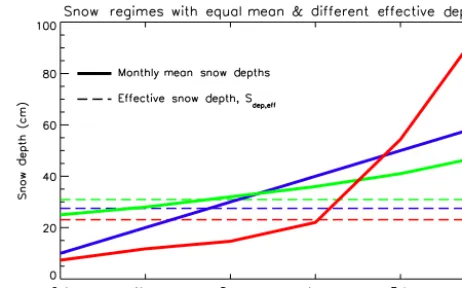
As shown in Fig. 1, a season with an early snowfall will typ-ically produce a higher effective snow depth than a linearly increasing snowpack with the same mean value. Similarly, if shallow snow persists for most of the winter but a large snowfall occurs in February, the effective snow depth will be lower than in the linear case.
Given inputs ofAnormandSdepth,eff(from observations or
models), we can efficiently compute the values of the three parameters P, Q, and R using a nonlinear fitting method (e.g., the Levenberg–Marquardt (LM) algorithm; Press et al., 2007). The relationship betweenAnormandSdepth,effinforms
us about the heat transfer mechanism between the atmo-sphere and the subsurface. To alleviate the problem of over-fitting, the curve is fit using data that are sampled evenly across a range of effective snow depths with up to 35 data points per 5 cm ofSdepth,effup to 50 cm (with the final
cate-gory being 45 cm or beyond). This sampling was performed 100 times, with the median of fit values taken; if the LM algo-rithm does not converge for a given sample, another sample is taken. Sampling also ensures that a wide variety of climatic regimes are used for characterizing the functional relation-ship seen in observations or a model.
3 Data
Assessing the relation between Anorm andSdepth,eff requires
three pieces of data: screen level air temperature, 20 cm soil temperature (as this is the most commonly observed depth), and snow depth. An analysis constraint is the need to use monthly mean values, as this is the most common output from large-scale land models.
A large network of hydrometeorological stations in Russia (and the former Soviet Union) provide the three required variables as follows: air temperature was acquired from the National Climatic Data Center (NCDC) Global Summary of the Day (https://data.noaa.gov/ dataset/global-surface-summary-of-the-day-gsod), provided the snow depths were measured at stations (as opposed to lo-cal transects), and information on soil temperatures is avail-able in Sherstyukov and Sherstyukov (2015). Data in the USA are from the Natural Resources Conservation Service as part of the SNOTEL and SCAN networks (http://www.
Figure 1.Effective snow depth (Sdepth,eff, dashed lines) of three
different snow regimes that have equal mean values over the period October–March. Earlier snowfall receives greater weighting as it represents greater insulation; data in green thus have the greatest effective depth.
wcc.nrcs.usda.gov/). In Canada, Alberta’s AgroClimate In-formation Service (ACIS; http://agriculture.alberta.ca/acis/) collates and distributes station data within the province.
For a given season, we use only sites with complete, quality-controlled records from October to March; 2049 ob-served site years are available. It is also recognized that the data have inherent limitations; for example it is unknown whether snow depths are measured at precisely the same lo-cation as the soil temperature measurements. Many measure-ments have been made on soils that have been historically al-tered; however our use of shallow (20 cm) soil temperatures and focus on the winter period aim to minimizes possible ar-tifacts due to disturbance.
Snow heat transfer in 13 models that participated in the CMIP5 experiment (Taylor et al., 2012; http://cmip-pcmdi. llnl.gov/cmip5/) is evaluated using the historical (1850– 2005) simulations. Soil columns within the various land models have different depths and layer thicknesses (Slater and Lawrence, 2013; their Fig. 2), so a spline interpolation of each monthly mean temperature profile was used to estimate a 20 cm value. Further details of the land models are available in Koven et al. (2013) and Slater and Lawrence (2013).
All data are restricted to those instances where, during the cooling period (October–March), meanTairis below−1◦C,
mean Tsoil is below 2.5◦C,Aair is greater than 10◦C, and Sdepth,effis greater than 1 cm and less than 150 cm. Observed
Locations with observed air and 20 cm soil temperature plus snow depth
Figure 2.Locations with colocated observations of air temperature,
20 cm soil temperature, and snow depth.
4 Results and discussion
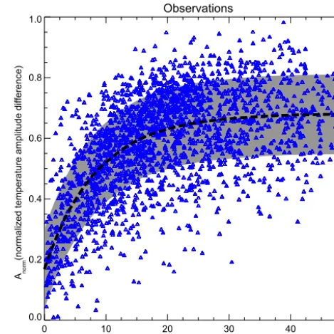
The observations show the expected exponential shape and fit the underlying theory (5) well despite significant scatter in the data (Fig. 3). The scatter likely arises from several sources, including (1) the range of climate conditions and snow regimes (Sturm et al., 1995) that occur across the land-scape, including the timing of snowfall and the pattern of snow metamorphism; (2) the properties and moisture content of the soil; and (3) uncertainties in the measurements them-selves and the measurement locations of the observed data. It is not possible to distinguish which of these sources of uncer-tainty dominates the scatter seen in Fig. 3, and it remains pos-sible that snowpack dynamics in regions outside the sampled data would generate slightly different relationships, though the shape of the curve would not likely change. Grey shading in Fig. 3 shows the span of median scatter of all 100 fits to the observations, with the black curve being the median fit value.
The observational results demonstrate that the marginal influence of snow insulation relative to the annual cycle of air temperature diminishes beyond a Sdepth,eff of about
25 cm. This phenomenon of insulation saturation has been previously noted in observations and models (Zhang, 2005; Lawrence and Slater, 2010).
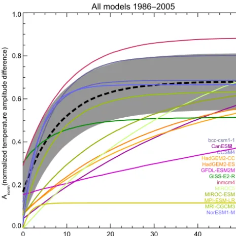
Results from models are calculated the same as observa-tions, with the median curve for each model shown on the same plot (Fig. 4). The difference amongst model curves is considerable. Several models produce an exponential-like curve (e.g., CCSM4, GISS, MRI, NorESM), suggesting that
Observations
0 10 20 30 40 50
Effective mean snow depth (cm) 0.0
0.2 0.4 0.6 0.8 1.0
Anorm
(normalized temperature amplitude difference)
Figure 3.Observed relation between Anorm and effective mean
snow depth (Sdepth,eff) along with the resulting exponential fit (dashed line). The grey shading shows the median fit plus/minus the mean scatter (Oerr)of all fits.
they generally reflect the character of the observed relation-ship. Many models, however, do not reproduce the observed relationship. Models such as CanESM, GFDL, Hadley mod-els, MIROC, and MPI are more linear in their form. This group of more poorly performing models all showAnorm
val-ues of less than 0.45 atSdepth,effof 20 cm (compared to a
me-dian observed value of 0.65 at 20 cm depth). A lowAnorm
value is produced when soil temperatures more closely track the changes in air temperature rather than being modulated by snow cover.
Note that the impact of heat transfer from the soil sur-face to 20 cm depth can be inferred from theAnorm values
atSdepth,eff=0 cm (Anorm typically between 0.05 and 0.30
atSdepth,eff=0 cm). Many models exhibit a lower
normal-ized temperature difference value atSdepth,eff=0 cm, which
suggests that these models are transferring heat through the upper soil too efficiently. The potential sources of a soil heat transfer bias are myriad and could be due to biases/errors in soil texture, soil moisture, soil water phase, soil thick-ness, and vegetation. Most of these models, apart from CLM (Lawrence and Slater, 2008), do not represent the highly in-sulative soil organic matter, so this is a potential explanation of the common biases atSdepth,eff=0 cm.
All models 1986–2005
0 10 20 30 40 50
Effective mean snow depth (cm) 0.0
0.2 0.4 0.6 0.8 1.0
Anorm
(normalized temperature amplitude difference)
bcc-csm1-1 CanESM2
CCSM4 HadGEM2-CC HadGEM2-ES GFDL-ESM2M GISS-E2-R inmcm4
MIROC5
MIROC-ESM
MPI-ESM-LR
MRI-CGCM3 NorESM1-M
Figure 4.Model fits to Eq. (5), showing large differences in how
heat is transferred though the snowpack to the soil. Data from the CMIP5 comparison period 1986–2005 are used. The dashed black line is the observational fit, with grey shading representing the ob-servational scatter as in Fig. 3.
al., 2001); hence insulation is not properly accounted for and cold temperatures easily penetrate into the soil. Conversely, the better-performing models feature multi-layer snowpacks that are more apt at emulating the nonlinear temperature pro-file of the snowpack. Note that the Hadley Centre model de-velopers have addressed this limitation by implementing a multi-layer snow model (Best et al., 2011; Chadburn et al., 2015).
Despite the application of a different coupled model component (e.g., atmosphere or ocean models) and differ-ent initial conditions, both of which will influence terres-trial surface climate, the two Hadley Centre climate models (HadGEM2-CC and HadGEM2-ES, both utilizing MOSES as their land model) produce essentially the same snow insu-lation curve. Similarly, CCSM4 and NorESM reproduce es-sentially the same curve, which is expected since both mod-els utilize CLM4 as their land model. The fact that snow insulation curves are essentially the same for a particular land model, even when driven with different climatic forc-ings from their parent climate model, suggests that the form of the curve does indeed capture the functional land model behavior.
The steep gradient ofAnormat shallowerSdepth,effis an
im-portant feature to capture as over 85 % of seasonally snow-covered land is estimated to have aSdepth,effless than 30 cm.
Reliable observed data of hemispheric-scale snow depths or mass is not yet available, but the prevalence of shallow
snow can be seen in estimated climatologicalSdepth,eff
de-rived from numerous reanalysis (ERA-Interim (Dee et al., 2011), MERRA (Rienecker et al., 2011), CFSR (Saha et al., 2010), JRA-55 (Kobayashi et al., 2015), some of which as-similate snow depths) products such as GlobSnow (Takala et al., 2011) and station interpolations (Foster and Davy, 1988; Brown and Brasnett, 2010) (Fig. 5).
A model diagnostic: the snow and heat transfer metric (SHTM)
A land model should be able to capture the exponential re-lationship betweenAnorm andSdepth,eff, and it is useful to
summarize the ability of a given model to do so as a com-pact metric. Here, we develop a snow and heat transfer met-ric (SHTM) that could be used within a broader land model analysis system such as the International Land Model Bench-marking project (ILAMB; http://www.ilamb.org; Luo et al., 2012). The metric is designed to have a value from 0 to 1 and describes the departure of a model’s snow insulation curve from the observed curve. As the marginal influence of snow insulation decreases after a Sdepth,eff value of about 25 cm
and most of the seasonal snow regions have aSdepth,effbelow
30 cm (Fig. 5), the SHTM value is only calculated over the range of 0 to 30 cm. For each 1 cm ofSdepth,eff, up to 30 cm,
twice the difference inAnorm between the model and
obser-vational curves is obtained; a root mean square error of these values is then computed and subtracted from 1. The SHTM value is thus
SHTM=1.− r
2·(ModelAnorm,i−ObservedAnorm,i) 2
.
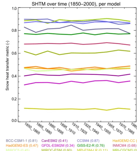
(7) The closer SHTM is to 1, the better the model is at repro-ducing the observed snow insulation curve; a lower limit of 0 is placed on the SHTM. An important feature of the SHTM is that it effectively isolates analysis of the snow in-sulation process and therefore should be robust across differ-ent climate forcing. We test that hypothesis here by calcu-lating the SHTM for ten 15-year periods from 1850 to 2000 for each model. The mean 2 m air temperature over the ter-restrial Northern Hemisphere north of 55◦N for the cooling period (October–March) was computed for each 15-year pe-riod for each model. As a measure of changing climates, the minimum and maximum of these 15-year averages was dif-ferenced per model, resulting in a span of 1.25 to 4.15◦C, with a mean of 2.15◦C. Despite these climatic changes, the
SHTM maintains a fairly constant value for each land model. Over the 150 years, all models return a SHTM standard de-viation of less than 0.021, which is substantially less than the typical SHTM difference between models and indicates a general invariance to climate variability (Fig. 6).
Figure 5.Cumulative distribution curves for climatological effec-tive snow depths (Sdepth,eff)as a percentage of all seasonally snow-covered area in the Northern Hemisphere (NH). The observed and model climatologies span a minimum of 10 years in the last quarter of the 20th century. The bold lines show the median values of the curves for both observations and models; shading shows the total range of curves. Note that the absolute snow-covered area can be quite different amongst models and observational estimates.
observational uncertainty, SHTM values within 0.05 of each other may not be significantly different, and incremental im-provements to the snow insulation schemes may not neces-sarily result in meaningful changes in the SHTM score. Ad-ditionally, the SHTM does not evaluate the ability of models to simulate snow accumulation or ablation; additional data sets and metrics are needed to assess these processes.
5 Conclusions
Model evaluation is an important aspect of the overall mod-eling process: e.g., development, application, and/or predic-tion. Land, hydrology, and ecology models can range in com-plexity from simpler, more conceptually based, formulations through to highly explicit representations that incorporate a multitude of processes. Regardless of their complexity, it is important that the underlying physical processes are repre-sented correctly.
Deriving the relationship between a normalized tempera-ture amplitude difference between air and soil, Anorm, and
the seasonal effective snow depth,Sdepth,eff, we have shown
that observations are consistent with heat transfer theory. Analysis of observed results suggests that the marginal im-pact of snow insulation diminishes beyond a Sdepth,eff of
about 25 cm. Structural weaknesses in several models have been exposed by examining their ability to represent the atmosphere–land heat transfer process in the presence of snow. To quantitatively compare model performance, a snow and heat transfer metric was designed. The SHTM value per model changed little when calculated for different periods over 150 years of climate change, suggesting it can fairly un-ambiguously provide an indication of whether model
struc-SHTM over time (1850–2000), per model
0.0 0.2 0.4 0.6 0.8 1.0
Snow heat transfer metric (-)
1850_18651865_18801880_18951895_19101910_19251925_19401940_19551955_19701970_19851985_2000
BCC-CSM1-1 (0.81) CanESM2 (0.41) CCSM4 (0.87) HadGEM2-CC (0.46)
HadGEM2-ES (0.47) GFDL-ESM2M (0.34) GISS-E2-R (0.76) INMCM4 (0.68) MIROC5 (0.45) MIROC-ESM (0.60) MPI-ESM-LR (0.11) MRI-CGCM3 (0.88) NorESM1-M (0.86)
Figure 6.Mean value of the snow and heat transfer metric (SHTM)
for each model. Values closer to 1.0 indicate better agreement with observations. SHTM values are relatively stable over 150 years of climate for each model.
tural/parameter deficiencies exist by negating other areas of uncertainty, such as the model forcing data. The SHTM is a useful model diagnostic that can be added to existing land model analysis/benchmarking systems.
Data availability. All data utilized in this study are publicly avail-able through the websites listed in Sect. 3.
Author contributions. Andrew G. Slater and David M. Lawrence conceived the idea. Andrew G. Slater conducted the analysis. An-drew G. Slater, David M. Lawrence, and Charles D. Koven wrote the manuscript.
Competing interests. The authors declare that they have no conflict of interest.
Acknowledgements. Among the authors, this work was supported by NSF PLR-1304152, PLR-1304220, NASA IDS project 1517544, and DOE DE-FC03-97ER62402/A010 and DE-AC02-05CH11231. Code for this method is to be implemented within the ILAMB system. Data sources and acknowledgements are given in the text.
Edited by: M. Schneebeli
References
Abramowitz, G., Leuning, R., Clark, M., and Pitman, A.: Evaluating the Performance of Land Surface Models, J. Clim., 21, 5468– 5481, doi:10.1175/2008JCLI2378.1, 2008.
Anisimov, O. A., Lobanov, V. A., Reneva, S. A., Shiklomanov, N. I., Zhang, T., and Nelson, F. E.: Uncertainties in grid-ded air temperature fields and effects on predictive active layer modeling, J. Geophys. Res.-Earth Surf., 112, F02S14, doi:10.1029/2006JF000593, 2007.
Best, M. J., Pryor, M., Clark, D. B., Rooney, G. G., Essery, R. L. H., Ménard, C. B., Edwards, J. M., Hendry, M. A., Porson, A., Gedney, N., Mercado, L. M., Sitch, S., Blyth, E., Boucher, O., Cox, P. M., Grimmond, C. S. B., and Harding, R. J.: The Joint UK Land Environment Simulator (JULES), model description – Part 1: Energy and water fluxes, Geosci. Model Dev., 4, 677–699, doi:10.5194/gmd-4-677-2011, 2011.
Brown, R. and Brasnett, B.: Canadian Meteorological Cen-tre (CMC) Daily Snow Depth Analysis Data. ©Environment Canada, 2010, Boulder, Colorado USA: National Snow and Ice Data Center, Digital media, 2010.
Chadburn, S. E., Burke, E. J., Essery, R. L. H., Boike, J., Langer, M., Heikenfeld, M., Cox, P. M., and Friedlingstein, P.: Impact of model developments on present and future simulations of permafrost in a global land-surface model, The Cryosphere, 9, 1505–1521, doi:10.5194/tc-9-1505-2015, 2015.
Clark, M. P., Fan, Y., Lawrence, D. M., Adam, J. C., Bolster, D., Gochis, D. J., Hooper, R. P., Kumar, M., Leung, L. R., Mackay, D. S., Maxwell, R. M., Shen, C., Swenson, S. C., and Zeng, X.: Improving the representation of hydrologic processes in Earth System Models, Water Resour. Res., 51, 5929–5956, doi:10.1002/2015WR017096, 2015.
Decker, M., Brunke, M. A., Wang, Z., Sakaguchi, K., Zeng, X., and Bosilovich, M. G.: Evaluation of the Reanalysis Products from GSFC, NCEP, and ECMWF Using Flux Tower Observations, J. Clim., 25, 1916–1944, doi:10.1175/JCLI-D-11-00004.1, 2012. Dee, D. P., Uppala, S. M., Simmons, A. J., Berrisford, P., Poli,
P., Kobayashi, S., Andrae, U., Balmaseda, M. A., Balsamo, G., Bauer, P., and Bechtold, P.: The ERA-Interim reanalysis: config-uration and performance of the data assimilation system, Q. J. Roy. Meteorol. Soc., 137, 553–597, doi:10.1002/qj.828, 2011. Dutta, K., Schuur, E. A. G., Neff, J. C., and Zimov, S. A.:
Po-tential carbon release from permafrost soils of Northeastern Siberia, Glob. Change Biol., 12, 2336–2351, doi:10.1111/j.1365-2486.2006.01259.x, 2006.
Ekici, A., Chadburn, S., Chaudhary, N., Hajdu, L. H., Marmy, A., Peng, S., Boike, J., Burke, E., Friend, A. D., Hauck, C., Krin-ner, G., Langer, M., Miller, P. A., and Beer, C.: Site-level model intercomparison of high latitude and high altitude soil thermal dynamics in tundra and barren landscapes, The Cryosphere, 9, 1343–1361, doi:10.5194/tc-9-1343-2015, 2015.
Essery, R. L. H., Best, M. J., and Cox, P. M.: MOSES 2.2 Technical Documentation, Hadley Centre technical note 30, 2001. Fisher, J. B., Sikka, M., Oechel, W. C., Huntzinger, D. N., Melton, J.
R., Koven, C. D., Ahlström, A., Arain, M. A., Baker, I., Chen, J. M., Ciais, P., Davidson, C., Dietze, M., El-Masri, B., Hayes, D., Huntingford, C., Jain, A. K., Levy, P. E., Lomas, M. R., Poulter, B., Price, D., Sahoo, A. K., Schaefer, K., Tian, H., Tomelleri, E., Verbeeck, H., Viovy, N., Wania, R., Zeng, N., and Miller, C. E.:
Carbon cycle uncertainty in the Alaskan Arctic, Biogeosciences, 11, 4271–4288, doi:10.5194/bg-11-4271-2014, 2014.
Foster, D. and Davy, R.: Global Snow Depth Climatology, US Air Force Enviro. Tech. Appl. Cent., Scott Air Force Base, Illinois, USA, 1988.
Gupta, H. V., Wagener, T., and Liu, Y.:Reconciling theory with ob-servations: elements of a diagnostic approach to model evalu-ation, Hydrol. Process., 22, 3802–3813, doi:10.1002/hyp.6989, 2008.
Hobbie, S. E., Schimel, J. P., Trumbore, S. E., and Randerson, J. R.: Controls over carbon storage and turnover in high-latitude soils, Glob. Change Biol., 6, 196–210, doi:10.1046/j.1365-2486.2000.06021.x, 2000.
Kobayashi, S., Yukinari, O. T. A., Harada, Y., Ebita, A., Moriya, M., Onoda, H., Onogi, K., Kamahori, H., Kobayashi, C., Miyaoka, K., and Takahashi, K.: The JRA-55 Reanalysis: General Specifi-cations and Basic Characteristics, J. Meteorol. Soc. Jpn. Ser II, 93, 5–48, doi:10.2151/jmsj.2015-001, 2015.
Koven, C., Riley, W., and Stern, A.: Analysis of permafrost thermal dynamics and response to climate change in the CMIP5 Earth System Models, J. Clim., 126, 1877–1900, doi:10.1175/JCLI-D-12-00228.1, 2013.
Koven, C. D., Schuur, E. A. G., Schädel, C., Bohn, T. J., Burke, E. J., Chen, G., Chen, X., Ciais, P., Grosse, G., Harden, J. W., Hayes, D. J., Hugelius, G., Jafarov, E. E., Krinner, G., Kuhry, P., Lawrence, D. M., MacDougall, A. H., Marchenko, S. S., McGuire, A. D., Natali, S. M., Nicolsky, D. J., Olefeldt, D., Peng, S., Romanovsky, V. E., Schaefer, K. M., Strauss, J., Treat, C. C., and Turetsky, M.: A simplified, data-constrained approach to es-timate the permafrost carbon-climate feedback., Philos. Transact. A Math. Phys. Eng. Sci., 373, doi:10.1098/rsta.2014.0423, 2015. Lawrence, D. M. and Slater, A. G.: Incorporating organic soil into a global climate model, Clim. Dyn., 30, 145–160, doi:10.1007/s00382-007-0278-1, 2008.
Lawrence, D. M. and Slater, A. G.: The contribution of snow con-dition trends to future ground climate, Clim. Dyn., 34, 969–981, doi:10.1007/s00382-009-0537-4, 2010.
Lawrence, D. M., Slater, A. G., and Swenson, S. C.: Simu-lation of Present-Day and Future Permafrost and Seasonally Frozen Ground Conditions in CCSM4, J. Clim., 25, 2207–2225, doi:10.1175/JCLI-D-11-00334.1, 2012.
Lawrence, D. M., Koven, C. D., Swenson, S. C., Riley, W. J., and Slater, A. G.: Permafrost thaw and resulting soil mois-ture changes regulate projected high-latitude CO2 and CH4 emissions, Environ. Res. Lett., 10, 94011, doi:10.1088/1748-9326/10/9/094011, 2015.
Luetschg, M., Lehning, M., and Haeberli, W.: A sensitivity study of factors influencing warm/thin permafrost in the Swiss Alps, J. Glaciol., 54, 696–704, doi:10.3189/002214308786570881, 2008.
Lunardini, V. J.: Heat Transfer in Cold Climates, Van Nostrand Reinhold, New York, 1981.
land models, Biogeosciences, 9, 3857–3874, doi:10.5194/bg-9-3857-2012, 2012.
Ménard, C. B., Ikonen, J., Rautiainen, K., Aurela, M., Arslan, A. N., and Pulliainen, J.: Effects of Meteorological and Ancillary Data, Temporal Averaging, and Evaluation Methods on Model Perfor-mance and Uncertainty in a Land Surface Model, J. Hydromete-orol., 16, 2559–2576, doi:10.1175/JHM-D-15-0013.1, 2015. Monson, R. K., Lipson, D. L., Burns, S. P., Turnipseed, A. A.,
De-lany, A. C., Williams, M. W., and Schmidt, S. K.: Winter forest soil respiration controlled by climate and microbial community composition, Nature, 439, 711–714, doi:10.1038/nature04555, 2006.
Mudryk, L. R., Derksen, C., Kushner, P. J., and Brown, R.: Char-acterization of Northern Hemisphere snow water equivalent datasets, 1981–2010, J. Climate, 28, 8037–8051, 2015. Prentice, I. C., Liang, X., Medlyn, B. E., and Wang, Y.-P.:
Re-liable, robust and realistic: the three R’s of next-generation land-surface modelling, Atmos. Chem. Phys., 15, 5987–6005, doi:10.5194/acp-15-5987-2015, 2015.
Press, W., Teukolsky, S., Vetterling, W., and Flannery, B.: Numer-ical Recipes: The Art of Scientific Computing, Cambridge Uni-versity Press, New York, 2007.
Rienecker, M. M., Suarez, M. J., Gelaro, R., Todling, R., Bacmeis-ter, J., Liu, E., Bosilovich, M. G., Schubert, S. D., Takacs, L., Kim, G.-K., Bloom, S., Chen, J., Collins, D., Conaty, A., da Silva, A., Gu, W., Joiner, J., Koster, R. D., Lucchesi, R., Molod, A., Owens, T., Pawson, S., Pegion, P., Redder, C. R., Reichle, R., Robertson, F. R., Ruddick, A. G., Sienkiewicz, M., and Woollen, J.: MERRA: NASA’s Modern-Era Retrospective Anal-ysis for Research and Applications, J. Climate, 24, 3624–3648, doi:10.1175/JCLI-D-11-00015.1, 2011.
Saha, S., Moorthi, S., Pan, H., Wu, X., Wang, J., Nadiga, S., Tripp, P., Kistler, R., Woollen, J., Behringer, D., Liu, H., Stokes, D., Grumbine, R., Gayno, G., Wang, J., Hou, Y., Chuang, H., Juang, H. H., Sela, J., Iredell, M., Treadon, R., Kleist, D., Van Delst, P., Keyser, D., Derber, J., Ek, M., Meng, J., Wei, H., Yang, R., Lord, S., Van Den Dool, H., Kumar, A., Wang, W., Long, C., Chelliah, M., Xue, Y., Huang, B., Schemm, J., Ebisuzaki, W., Lin, R., Xie, P., Chen, M., Zhou, S., Higgins, W., Zou, C., Liu, Q., Chen, Y., Han, Y., Cucurull, L., Reynolds, R. W., Rutledge, G., and Goldberg, M.: The NCEP Climate Forecast System Reanalysis, B. Am. Meteorol. Soc., 91, 1015–1057, doi:10.1175/2010BAMS3001.1, 2010.
Schuur, E., McGuire, A., Schaedel, C., Grosse, G., Harden, J., Hayes, D., Hugelius, G., Koven, C., Kuhry, P., Lawrence, D., Na-tali, S., Olefeldt, D., Romanovsky, V., Schaefer, K., Turetsky, M., Treat, C., and Vonk, J.: Climate change and the permafrost car-bon feedback, Nature, 520, 171–179, doi:10.1038/nature14338, 2015.
Sharratt, B., Baker, D., Wall, D., Skaggs, R., and Ruschy, D.:Snow Depth Required for Near Steady-State Soil Temperatures, Agric. For. Meteorol., 57, 243–251, doi:10.1016/0168-1923(92)90121-J, 1992.
Sherstyukov, A. B. and Sherstyukov, B. G.: Spatial features and new trends in thermal conditions of soil and depth of its sea-sonal thawing in the permafrost zone, Russ. Meteorol. Hydrol., 40, 73–78, doi:10.3103/S1068373915020016, 2015.
Slater, A. G.: Surface Solar Radiation in North America: A Com-parison of Observations, Reanalyses, Satellite, and Derived Prod-ucts, J. Hydrometeorol., 17, 401–420, doi:10.1175/JHM-D-15-0087.1, 2016.
Slater, A. G. and Lawrence, D. M.: Diagnosing Present and Future Permafrost from Climate Models, J. Climate, 26, 5608–5623, doi:10.1175/JCLI-D-12-00341.1, 2013.
Slater, A. G., Schlosser, C. A., Desborough, C. E., Pitman, A. J., Henderson-Sellers, A. A., Robock, A. A., Vinnikov, K., Entin, J. J., Mitchell, K. K., Chen, F. F., Boone, A. A., Etchevers, P. P., Habets, F. F., Noilhan, J. J., Braden, H. H., Cox, P. M., de Rosnay, P. P., Dickinson, R. E., Yang, Z. L., Dai, Y. J., Zeng, Q. Q., Duan, Q. Q., Koren, V. V., Schaake, S. S., Gedney, N. N., Gusev, Y. M., Nasonova, O. N., Kim, J. J., Kowalczyk, E. A., Shmakin, A. B., Smirnova, T. G., Verseghy, D. D., Wetzel, P. P., and Xue, Y. Y.: The representation of snow in land surface schemes: Results from PILPS 2(d), J. Hydrometeorol., 2, 7–25, doi:10.1175/1525-7541(2001)002<0007:TROSIL>2.0.CO;2, 2001.
Sturm, M., Holmgren, J., and Liston, G. E.: A seasonal snow cover classification system for local to global applications, J. Clim., 8, 1261–1283, doi:10.1175/1520-0442(1995)008, 1995.
Takala, M., Luojus, K., Pulliainen, J., Derksen, C., Lemmetyi-nen, J., Karna, J.-P., KoskiLemmetyi-nen, J., and Bojkov, B.: Estimating northern hemisphere snow water equivalent for climate research through assimilation of space-borne radiometer data and ground-based measurements, Remote Sens. Environ., 115, 3517–3529, doi:10.1016/j.rse.2011.08.014, 2011.
Taylor, K. E., Stouffer, R. J., and Meehl, G. A.: An Overview Of CMIP5 And The Experiment Design, B. Am. Meteorol. Soc., 93, 485–498, doi:10.1175/BAMS-D-11-00094.1, 2012.
Yershov, E.: General Geocryology, Cambridge University Press, 1998.
Yi, Y., Kimball, J. S., Rawlins, M. A., Moghaddam, M., and Eu-skirchen, E. S.: The role of snow cover affecting boreal-arctic soil freeze-thaw and carbon dynamics, Biogeosciences, 12, 5811– 5829, doi:10.5194/bg-12-5811-2015, 2015.