Atmos. Meas. Tech., 6, 99–103, 2013 www.atmos-meas-tech.net/6/99/2013/ doi:10.5194/amt-6-99-2013
© Author(s) 2013. CC Attribution 3.0 License.
Atmospheric
Measurement
Techniques
Improving Langley calibrations by reducing diurnal variations of
aerosol ˚
Angstr¨om parameters
A. Kreuter, S. Wuttke, and M. Blumthaler
Division for Biomedical Physics, Department of Physiology and Medical Physics, Innsbruck Medical University, Muellerstr. 44, 6020 Innsbruck, Austria
Correspondence to: A. Kreuter ([email protected])
Received: 25 July 2012 – Published in Atmos. Meas. Tech. Discuss.: 7 September 2012 Revised: 18 December 2012 – Accepted: 1 January 2013 – Published: 14 January 2013
Abstract. Errors in the sun photometer calibration constant lead to artificial diurnal variations, symmetric around solar noon, of the retrieved aerosol optical depth (AOD) and the associated ˚Angstr¨om exponent α and its curvature γ. We show in simulations that within the uncertainty of state-of-the-art Langley calibrations, these diurnal variations ofαand
γ can be significant in low AOD conditions, while those of AOD are negligible. We implement a weighted Monte Carlo method of finding an improved calibration constant by minimizing the diurnal variations inαandγ and apply the method to sun photometer data of a clear day in Innsbruck, Austria. The results show that our method can be used to im-prove the calibrations in two of the four wavelength channels by up to a factor of 3.6.
1 Introduction
Sun photometers (SPM) are radiometers to determine the spectral aerosol optical depth (AOD), the columnar aerosol loading of the atmosphere, which is an important radiative forcing parameter of the Earth’s climate system (Forster et al., 2007). The AOD is determined from direct sun irradiance measurements and application of the Bouguer–Lambert– Beer law which describes the exponential extinction of light on its way through the atmosphere. The main challenges in sun photometry are the calibration as well as ensuring a con-stant filter transmission (Shaw, 1976).
The best sun photometer calibration methods are the so-called Langley calibrations (and its variations), which are based on extrapolating the diurnal SPM signal to zero air mass (e.g. Forgan, 1994). While no additional equipment is
needed, the Langley methods require clear and highly stable atmospheric aerosol conditions, typically only found above the planetary boundary layer on high mountain sites.
Here, we introduce a new method that may alleviate this restriction and improve the SPM calibration beyond the Lan-gley uncertainty.
2 Systematic diurnal variations of AOD and ˚
Angstr¨om parameters
A ground-based photo detector pointed at the sun with a nar-row field-of-view and a band pass filter measures a signalV
that is related to the signal at the top of the atmosphereV0
(the calibration constant, sometimes also called extraterres-trial signal) by
V =V0/r2×exp(−τ m), (1)
where r is the normalized Sun–Earth distance and m is the relative air mass factor. The air mass is approximately 1/cos(θ ),θ is the solar zenith angle (SZA), and refined ex-pressions are given by Kasten and Young (1989). The total extinctionτ is the sum of the contributions of aerosol optical depthτa andτray, the extinction due to molecular Rayleigh
scattering (Bodhaine et al., 1999). Here, for simplicity and clarity of the argument, we restrict the discussion to bands outside molecular absorptions.
The logarithm of the signalV has a linear diurnal depen-dency on the air mass with slope τ and ordinate intercept log (V0/r2). So the calibration constantV0can be found by a
100 A. Kreuter et al.: Improving Langley calibrations
at high mountain sites (e.g. Mauna Loa, Hawaii or Jungfrau-joch, Swiss Alps) are amongst the most accurate methods for SPM calibration and achieve uncertainties below 0.5 % (Hol-ben et al., 1998; Schmid et al., 1998; Wehrli, 2000).
KnowingV0, the AOD can be calculated straightforwardly
by rearranging Eq. (1):
τa= −log(r2V /V0)/m−τray. (2)
Errors in the calibration are typically the largest sources of uncertainty in determining AOD (Shaw, 1976). It follows from Eq. (2) that an error in V0causes an air mass
depen-dent offset in the derived AOD, which has been pointed out by several authors (see, e.g. Cachorro et al., 2008). The er-roneously derived AOD,τa0under the assumption of a wrong
V00is
τa0=τa+log(V00/V0)/m. (3)
A calibration error manifests itself in an artificial diurnal variation (DV) of the derived AOD. The deviation has a max-imal magnitude at noon (bigger for higher solar elevations) and vanishes for large air masses at sunset/sunrise and is symmetrical around local solar noon. Cachorro et al. (2008) have proposed an improvement of the calibration from that effect, but like all variations of the Langley method, it is in-trinsically limited by the natural variations of AOD.
Here we consider the spectral AOD relation because it is not affected by AOD variations if the aerosol type does not change. The AOD dependency on wavelength is usually de-scribed by the ˚Angstr¨om exponentα( ˚Angstr¨om, 1964). With
˚
Angstr¨om’s power-law ansatz, the logτa−logλrelationship
is linear with slopeα:
logτa=logβ−αlogλ, (4)
withλin units of microns, and whereβis the AOD at wave-length of one micron. It has become common (e.g. Schuster et al., 2006) to add a quadratic term in logλto account for a possible curvature:
logτa=logβ∗+α∗logλ+γlog2 λ. (5)
The parameters α and γ are determined by regression of Eqs. (4) and (5), respectively. To investigate the sensitivity of AOD,αandγ on the calibration, we theoretically simulate the SPM measurement and retrieval process. We consider the case of the precision filter radiometer SPM (PFR-SPM) developed by the Physikalisch-Meteorologisches Observato-rium (PMOD) in Davos, Switzerland, for the Global Atmo-spheric Watch Network (Wehrli, 2000). It features four stan-dard aerosol wavelength channels: 368 nm, 412 nm, 501 nm and 862 nm, which will be referred to as channels 1 to 4, respectively. For comparison, commonly used wavelengths measured by the AErosol RObotic NETwork are 380 nm, 440 nm, 500 nm, 670 nm and 870 nm (Holben et al., 1998).
We simulate the diurnal signalV for all wavelengths for a given spectral τa using Eq. (1) and a hypothetical wrong
calibration constantV00of channel 4 at 862 nm ofV0+σ and
V0−σ, whereσis the calibration uncertainty of 0.5 %. From
Eq. (2) we derive the erroneous spectral AODτa0under the as-sumption ofV00=V0, from which we obtain the (erroneous)
α0andγ0.
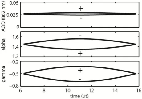
Figure 1 shows the calculation for the example values:
β∗=0.02,α∗=2, andγ = −0.5, which constitute pristine conditions. The time (UT) corresponds to a SZA between 87◦ and 63◦or air mass between 23 and 2.2 at noon (11:25 UT), beginning of November at the location of Innsbruck, Austria, at 11◦E and 47◦N.
All parameters show the characteristic DV symmetric around noon. The deviation of AOD,αandγ is biggest at local noon (DV amplitude) and approaches the correct val-ues at low solar elevation. The respective effect ofV0+σ
andV0−σ traces two branches marking the bounds of
pos-sible DVs, which are statistically allowed by the calibration uncertainty.
The example reveals that the DV inα and, in particular,
γ can be considerable, even ifV00 lies within theV0
uncer-tainty. The DV amplitude ofαandγ can reach 0.1 and 0.2, respectively. The amplitude of the DV in AOD (∼0.002 for channel 4) is negligibly small and will likely be obscured by natural variations.
This DV inαandγ is also of specific relevance as these parameters are used as indicators of the size or size distri-bution of aerosols. King et al. (1978) have introduced a nu-merical inversion of the spectral AOD to obtain the aerosol size distribution. A semiquantitative graphical method has been proposed (Schuster et al., 2006, and Gobbi et al., 2007), where γ (or equivalently, the α-difference dA) is plotted against α. Changes in fine mode size and fraction trace curved lines of a grid. Since here we use the more uni-versal parameter of the curvature γ instead of dA, we call this alpha–gamma representation AGa-plot (in allusion to the AdA-plot in Gobbi’s nomenclature).
With its appealing simplicity, this representation reveals, for example, diurnal aerosol evolution such as humidification or drying. In this context, calibration errors and resulting ar-tificial DVs ofαandγare specifically relevant, because they modify the AGa-plot and its interpretation.
The individual effect of a calibration error in each of the different channels on the AGa-plot is illustrated in Fig. 2. Each colored line represents the resulting DV when adding an error of 1σ (0.5 %) to theV0of the respective channel.
A. Kreuter et al.: Improving Langley calibrations 101
12
Figures
274
Fig.1
275
276
Fig.2
277
278
Fig.3
279
280
Fig. 1. Simulated DV of AOD0,α0andγ0for a calibration error in PFR-SPM channel 4 ofV00=V0+σandV0−σ, respectively.
3 Minimization of Diurnal Variations
As demonstrated, a residual artificial DV inαandγmay per-sist even after state-of-the-art calibration, showing that these parameters are extremely sensitive to calibration errors. The idea here is to harness this sensitivity and improve the cali-bration by minimizing any residual DV inαandγ. Conse-quently, this also improves the accuracy of the AGa represen-tation and its interprerepresen-tation. The question is, can one find a set ofV0for all channels as close as possible to the certified
calibration so that DVs inαandγboth vanish?
We propose to solve the problem with a conceptually sim-ple Monte Carlo (MC) method: trying a large ensemble of random combinations ofV00weighted with a Gaussian uncer-tainty function centered onV0, and select theV00 that yields
the smallest DV. Since bothαandγshow independent DVs, we consider the total DV (TDV) amplitude to be minimized: TDV2= DV2α+ DV2γ. The DV amplitudes DVα and DVγ are specified here as their respective difference of their values at noon (lowest SZA) and highest SZA. An ensemble of diur-nalαandγvalues from 100 generatedV00is shown in Fig. 2. The DVs are arranged in a “star” pattern, with the center be-ing the trueαandγvalues approached at low solar elevation and the length of the spikes are the TDV amplitudes.
Note that using a random number forV00 that is normally distributed withσ is an implicit weighting of the solution by the mean squared error ofV0andV0best. Smaller deviations
ofV00fromV0are more likely generated in the MC method,
and hence the solutionV0best should be found as close toV0
as possible.
4 Application to SPM data
We then apply the above MC method of finding an improved
V0 with resulting minimal TDV to real data of our SPM
12
Figures
274
Fig.1
275
276
Fig.2
277
278
Fig.3
279
280
Fig. 2. Calibration error effect in the AGa representation ofV00=
V0+σ in each individual PFR-SPM channel (colored lines) and that of an ensemble of 100 normally distributed randomV0errors
in all channels (black lines).
located in Innsbruck, Austria. We have been measuring AOD since 2007 and the 5-yr climatology has recently been pub-lished (Wuttke et al., 2012).
The SPM has been calibrated at the PMOD by comparison with two Langley calibrated standard instruments.V0for the
four wavelengths channels from the certificate is
V0C=(4.262(20) 3.778(16) 3.772(30) 3.565(20)) V , (6) where the 1σuncertainties are given in brackets, correspond-ing to relative accuracies inV0 of 0.5 %, 0.4 %, 0.8 % and
0.6 %, respectively.
We found a particularly good example day in Innsbruck with low and fairly constant AOD on 10 November 2011. This cloudless day in late autumn with relatively low so-lar elevation was characterized by a dominant anticyclonic weather situation, no wind and no convective mixing of the boundary layer.
We define DVα as the difference ofα at noon (mean of 24 min) and the mean of α at three hours before and after noon. DVγ is defined accordingly and again the TDV am-plitude is considered. We run the MC procedure with 10 000 trials (different combinations of weighted randomV00) to se-lect theV00with the minimal TDV amplitude and find
102 A. Kreuter et al.: Improving Langley calibrations
12
Figures
274
Fig.1
275276
Fig.2
277278
Fig.3
279280
Fig. 3. (a) SPM data of 10 November 2011 used for improving the calibration by minimizing the TDV amplitude with a MC method. The
difference of retrieved AOD withV0C(red) and the newV0best(green) is within the measurement uncertainty. (b) The effect of the improved calibration on the AGa-plot is significant. Notably, the green points are more clustered and shifted to a largerγ value. The grid lines refer to fine mode radius (µm) and fraction (%).
AODs (variation) over the day of each channel (except for channel 3 where the standard deviation of AOD is 0.03). No significant DV of AOD can be detected within the natural fluctuations.
The data for α and γ are depicted in the AGa-plot in Fig. 3b. The original DV (red dots) inγ is significant, as it ranges from−0.4 in the morning to−0.9 at noon. The vari-ation inαis less and ranges from 1.5 to 1.6. Consequently, in the AGa-plot the representation has changed significantly after application ofV0best. The loci of green points are now more clustered (standard deviations ofαandγ are 0.02 and 0.03, respectively) and indicate a largerγ, pointing towards a smaller fine mode radius and fraction.
5 Discussion
One of the questions after finding a solution with minimal TDV and correspondingV0best is about its uniqueness. One might conclude that aV00 that minimizes the TDV is neces-sarily closer to the trueV0. This seems not true in general.
The calibration error in each channel results in a different TDV, both in magnitude and direction in the AGa representa-tion (Fig. 2). This means that a given TDV can be realized by a variety of combinations inV00, and hence, the sole criterion of a minimal TDV does not yield a unique solutionV0best. It is only the result of the additional constraint of minimizing the root-mean-squared error (rms) with respect to the origi-nalV0(realized by the normal distribution of trials in the MC
method) that a unique solution can be found. Of course, for aV0bestwith a large rms distance to the true calibration, the DV in the AOD will become significant and can then be used as a constraint.
The next question is about the uncertainty of the solution
V0best and whether it really constitutes an improvement be-yond the Langley uncertainty. We repeat the MC procedure
with 100 trials of simulated data for 100 randomV0in the
in-terval (V0−σ,V0+σ) and compare each solutionV0bestwith
the corresponding target inputV0. The standard deviation of
the difference of the two is the uncertainty ofV0best. We find that channels 1 and 2 have similar standard deviations as the
σ of 0.5 %. The standard deviation of channels 3 and 4 are determined to 0.31 % and 0.14 %, respectively. This implies that theV0best of channels 3 and 4 are indeed closer to the trueV0and reduce their calibration uncertainty to 0.61σ and
0.28σ, respectively.
The reason why the channels at higher wavelengths are more sensitive here, is that their wavelength spacing (in log-arithmic scale) increases with wavelength. The loglog-arithmic distance between channels 1 and 2 is 1/5 of that of channel 3 and 4. The latter are hence more influential on the determi-nation ofαandγ, and their calibration is more sensitive.
The reduction of the calibration uncertainty achieved here stems from the consideration of the spectral AOD, i.e. the combination of all channels as opposed to each channel indi-vidually in the Langley methods. The spectral AOD relations are more sensitive to calibration errors and independent of natural AOD variations. Langley conditions (constant AOD) are hardly met at low elevation stations, while constant spec-tral AOD conditions do occur more frequently. This is an empirical observation based on our aerosol climatology in Innsbruck, and we do not see any principal reason why it should not be more generally applicable to other stations. On suitable days for this method, such as our example day, the residual variation inαandγ should be small after minimiz-ing the TDV (green points in Fig. 3b).
A. Kreuter et al.: Improving Langley calibrations 103
6 Conclusions
We have shown that the ˚Angstr¨om parametersαandγ are extremely sensitive indicators of calibration errors and ar-tificial DVs can be significant under low AOD conditions, even if the calibration is within 0.5 % relative uncertainty. The DV amplitudes inαandγ can be reduced by stochas-tically varying the calibration constantV0using a weighted
MC method. The method has been characterized with model simulations and applied to real data from a PFR-SPM on a clear and stable day in Innsbruck. Minimizing the total DV amplitude inαandγ, a new calibration constantV0has been
determined which reduces the calibration uncertainty of two of the PFR-SPM wavelengths channels by a factor of up to 3.6. Our method may be easily generalized to other SPMs with more and/or different aerosol wavelength channels to improve the calibration beyond the Langley uncertainty.
Acknowledgements. We thank G.P. Gobbi for the calculation of the
grid lines in the AGa-plots. Edited by: S. Schmidt
References
˚
Angstr¨om, A.: The parameters of atmospheric turbidity, Tellus, 16, 64–75, 1964.
Bodhaine, B. A., Wood, N. B., Dutton, E. G., and Slusser, J. R.: On Rayleigh Optical Depth Calculations, J. Atmos. Ocean. Tech. 16, 1854–1861, 1999.
Cachorro, V. E., Toledano, C., Berjon, A., de Frutos, A. M., Torres, B., Sorribas, M., and Laulainen, N. S.: An “in situ” calibration-correction procedure (KCICLO) based on AOD diurnal cycle: Comparative results between AERONET and reprocessed (KCI-CLO method) AOD-alpha data series at El Arenosillo, Spain, J. Geophys. Res. 113, D02207, doi:10.1029/2007JD009001, 2008.
Forgan, B. W.: General method for calibrating Sun photometers, Appl. Optics, 33, 4841–4850, 1994.
Forster, P., Ramaswamy, V., and Artaxo, P., et al.: Changes in At-mospheric Constituents and in Radiative Forcing, in: Climate Change 2007: The Physical Science Basis, Contribution of WG I to the Fourth AR of the IPCC, Cambridge University Press, Cambridge, United Kingdom and New York, NY, USA, 2007. Gobbi, G. P., Kaufman, Y. J., Koren, I., and Eck, T. F.: Classification
of aerosol properties derived from AERONET direct sun data, Atmos. Chem. Phys., 7, 453–458, doi:10.5194/acp-7-453-2007, 2007.
Holben, B. N., Eck, T.F., Slutsker, I., Tanre, D., Buis, J. P., Set-zer, A., Vermote, E., Reagan, J. A., Kaufman, Y. J., Nakajima, T., Lavenu, F., Jankowiak, I., and Smirnov, A.: AERONET- A federated instrument network and data archive for aerosol char-acterization, Remote Sens. Env., 66, 1–16, doi:10.1016/S0034-4257(98)00031-5, 1998.
Kasten, F. and Young, A. T.: Revised optical air mass tables and approximation formula, Appl. Optics, 28, 4735–4738, 1989. King, M. D., Byrne, D. M., Herman, B. M., and Reagan, J. A.:
Aerosol Size Distributions Obtained by Inversion of Spectra Op-tical Depth Measurements, J. Atmos. Sci. 35, 2153–2167, 1978. Schmid, B., Spyak, P. R., Biggar, S. F., Wehrli, C., Sekler, J., Ingold, T., M¨atzler, C., and K¨ampfer, N.: Evaluation of the applicability of solar and lamp radiometric calibrations of a precision Sun pho-tometer operating between 300 and 1025 nm, Appl. Optics, 37, 3923–3941, 1998.
Schuster, G. L., Dubovik, O., and Holben, B. N.: ˚Angstr¨om expo-nent and bimodal aerosol size distributions, J. Geophys. Res., 111, 1–14, doi:10.1029/2005JD006328, 2006.
Shaw, G. E.: Error analysis of multi-wavelength sun photometry, Pure Appl. Geophys., 114, 1–14, 1976.
Wehrli, C.: Calibrations of filter radiometers for determination of atmospheric optical depth, Metrologia, 37, 419–422, 2000. Wuttke, S., Kreuter, A., and Blumthaler, M.: Aerosol