Flexible Performance Prediction of Data Center Networks
using Automatically Generated Simulation Models
∗Piotr Rygielski
Chair of Software EngineeringSamuel Kounev
Chair of Software EngineeringPhuoc Tran-Gia
Chair of CommunicationNetworks
Institute of Computer Science, University of Würzburg, Am Hubland, 97074 Würzburg, Germany
{piotr.rygielski@, samuel.kounev@, trangia@informatik.}uni-wuerzburg.de
ABSTRACT
Using different modeling and simulation approaches for pre-dicting network performance requires extensive experience and involves a number of time consuming manual steps re-garding each of the modeling formalisms. In this paper, we propose a generic approach to modeling the performance of data center networks. The approach offers multiple perfor-mance models but requires to use only a single modeling language. We propose a two-step modeling methodology, in which a high-level descriptive model of the network is built in the first step, and in the second step model-to-model transformations are used to automatically transform the de-scriptive model to different network simulation models. We automatically generate three performance models defined at different levels of abstraction to analyze network through-put. By offering multiple simulation models in parallel, we provide flexibility in trading-off between the modeling ac-curacy and the simulation overhead. We analyze the sim-ulation models by comparing the prediction accuracy with respect to the simulation duration. We observe, that in the investigated scenarios the solution duration of coarser simu-lation models is up to 300 times shorter, whereas the average prediction accuracy decreases only by 4 percent.
Categories and Subject Descriptors
C.4 [Performance of Systems]: Modeling techniques
Keywords
performance modeling, data center networks, meta-modeling
1.
INTRODUCTION
Performance modeling and prediction approaches help sys-tem operators to analyze data center performance at syssys-tem design-time and during operation. Nowadays, data centers ∗This work is a part of RELATE project supported by the European Commission (Grant no. 264840ITN).
.
are becoming increasingly big and dynamic due to the com-mon adoption of virtualization technologies. Virtual ma-chines, data, and services can be migrated on demand be-tween physical hosts to optimize resource utilization while enforcing service-level agreements. This makes an accurate and timely performance analysis a challenging problem [17]. In our research, we focus on the network infrastructures of modern virtualized data centers. Network infrastructures in such environments introduce several new challenges for performance analysis. Some examples of such challenges in-clude the growing density of modern virtualized data centers (increasing amount of network end-points), the high volume of intra-data-center traffic (having its source and destina-tion within the same data center), or the new traffic sources introduced in the management layer of virtualized environ-ments (e.g., migration of virtual machines).
Computer networks can be represented in multiple perfor-mance modeling formalisms, as for example, domain-specific simulation models, stochastic Petri nets, queueing networks, and stochastic process algebras. The use of a given perfor-mance model requires understanding of its formalism and the usual modeling steps. Thus, specific knowledge and ex-perience with the various modeling formalisms are required in order to benefit from their different characteristics. Usu-ally, such knowledge and experience is missing or it is limited to a single modeling formalism.
We propose an approach that requires to model the net-work using a high-level descriptive language that is generic and contains elements familiar to any network operator. That approach enables the use of multiple different mod-eling and analysis approaches without requiring in depth expertise in the respective modeling formalisms. Using the high-level descriptive model as a basis, we provide model-to-model transformations to automatically generate predictive performance models without requiring the operator to have expertise in any of them. For the descriptive modeling of the network infrastructure, we use the Descartes Network Infrastructure (DNI) meta-model as a part of the Descartes Modeling Language (DML) [9]. We refer to meta-models as to modeling languages specified using the MOF formalism (Meta-object Facility) [3]. Network models that are built us-ing theDNI modeling language can be automatically trans-formed to various predictive models; in this paper we present three predictive models that can be automatically derived: OMNeT++ simulation and two different stochastic models based on Queueing Petri Nets (QPN).
The main contributions of this paper are the following. (i) We propose two new model transformations to
automat-SIMUTOOLS 2015, August 24-26, Athens, Greece Copyright © 2015 ICST
ically generate performance models based on a single de-scriptive DNI model instance that is given as an input. (ii) As an intermediate step, we propose a newminiDNI meta-model that is smaller thanDNI and offers coarser modeling granularity. Transformation fromDNI to miniDNI is per-formed automatically, so only an instance of theDNI must be provided at the input. (iii) We compare the three predic-tive models against existing performance models obtained by using theDNI model and the previous transformations partially introduced in [27, 29]. We reveal the semantic gaps between the model abstractions and the different model solv-ing techniques. (iv) We evaluate the three predictive mod-els with respect to their performance prediction accuracy and the time needed to solve them. Finally, we discuss the results, describe technical challenges, and characterize sit-uations in which a given simulation model performs better than the other models.
The novelty of our approach can be characterized by the following aspects. First, we propose an original descriptive performance modeling language that offers automatic trans-formation to performance predictive models for performance prediction. Second, thanks to the technology-independence of the DNI modeling language, our approach can be used for modeling novel networking technologies such as network virtualization, and flow-based routing. Third, from a sin-gle DNI network model, we automatically provide multiple predictive models that offer different modeling granularity, prediction accuracy, and model solution time. This allows a flexible selection of the prediction model according to the required prediction accuracy and time constrains (e.g., pre-diction within max. 3 minutes). Fourth, we cover the end-to-end performance specifications of the modern data cen-ters by supporting generic server and network virtualization and the link to the deployed software. We do not focus on selected fragments of a specific protocol but model the net-work as a whole including the deployed software, physical and virtual topology, configuration and traffic.
The rest of this paper is organized as follows. In Section 2, we introduce the foundations, briefly reviewing network per-formance modeling formalisms and related perper-formance pre-diction approaches. In Section 3, we introduce our approach to performance modeling and prediction. Section 4 briefly presents the descriptive models and the different model-to-model transformations. Additionally, we characterize the differences between the generated predictive models. In Sec-tion 5, we present our evaluaSec-tion of the predicSec-tion accuracy and the simulation overhead. We describe the model cal-ibration process and formulate technical challenges related to it. Finally, we present our plans for future works and conclude the paper in Section 6.
2.
FOUNDATIONS AND RELATED WORK
There is a large body of existing work on performance modeling of communication networks. The related work can be divided into two main areas: predictive models for perfor-mance analysis and approaches that rely on the model-based generation of predictive models.
2.1
Performance Models for Data Center
Net-works
There exist many performance modeling formalisms suit-able for modeling networks, for example [16, 25]. Existing modeling approaches are mostly based on stochastic models
such as classical product-form queueing networks, layered queueing networks, stochastic Petri nets, stochastic simula-tion models, and so on. We can distinguish domain-specific performance models (e.g., network simulators) and general purpose models that can be used to model the networks.
The most popular network simulation frameworks are OM-NeT++ [31] and ns-2/3 [26] — both discrete event simula-tors. In [26], ns-2 has been claimed for many years to be standard simulator for academic network research. Model-ing usModel-ingns-2 requires extensive knowledge of programming in C++ and thus required time investment to learn how to model. Similar observations apply to OMNeT++—almost all protocol-specific models need to be implemented by hand. According to [34], further similar simulators include: open-WNS, OPNET, GTNetS, and IKR simulation library. All these simulators focus on medium-detailed modeling of the popular TCP/IP protocol stacks; extensions to support fur-ther popular protocols are often available as well. There exist also simulators that are tightly bound to a given pro-tocol or even to a concrete implementation of that propro-tocol. An example is the Venus simulator [12]; the authors use the TCP implementation extracted from FreeBSD v9 kernel to keep the simulation accuracy maximized.
On the other hand, there exist general-purpose perfor-mance modeling formalisms that can also be applied for net-work modeling. To such formalisms we account, for example, queueing networks, layered queueing networks, stochastic Petri nets, stochastic process algebras, Markov chains, ana-lytical estimation methods (bounds analysis). In [25], Puig-janer reviewed selected general-purpose performance model-ing formalisms and their applicability in the communication networks area.
In this paper, we use, among others, stochastic Petri nets as a predictive model. Regarding the stochastic Petri nets, such as queueing Petri nets, and their usage in a network-ing context, so far they have mainly been used to model specific network components at a high level of detail but with limited scope as, for example in [37, 21]. However, an end-to-end modeling approach is crucial in modern virtual-ized systems. The authors of [33] claim:
”The fundamental problem is that the simple textbook end-to-end delay model composed of network transmission delay, propagation delay, and router queueing delay is no longer sufficient. Our results show that in the virtualized data center, the delay caused by end host virtualization can be much larger than the other delay factors and cannot be overlooked.”
Domain-specific simulators cover in high detail selected performance-relevant aspects of communication networks. To the other extreme—regarding the level of abstraction of the models—we account black-box approaches, where the performance metrics of interest are calculated using simple mathematical equations based on a few general network pa-rameters. The black-box modeling approach is normally ap-plied in cases where the networks are not in the main focus of the analysis, but their influence on performance cannot be neglected. Such approaches can be found in [14, 20].
2.2
Approaches based on Model-to-model
Transformations
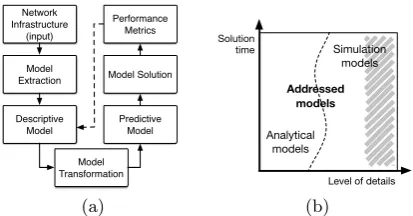
Network Infrastructure
(input)
Descriptive Model
Model Transformation
Predictive Model Model Solution Model
Extraction
Performance Metrics
(a)
Level of details Solution
time Simulation models
Analytical models
Addressed models
(b)
Figure 1: (a) Process of performance prediction based on model-to-model transformations. (b) Ab-stract division of prediction models into analytical and simulation models. Models with very fine mod-eling granularity (gray area) are not our target.
and all predictive models are derived automatically using model transformations. The general performance prediction process based on model-to-model transformations is pre-sented in Figure 1a. A model of a real network is built and stored in a descriptive model with performance annota-tions, whereas the rest of the process is automated and can deliver as many different predictive performance models as many model transformations are available. Some authors, e.g., [23], use the prediction results to further refine their models (dashed line in Fig. 1a).
Approaches based on model-to-model transformations stem from software engineering community. UML models are used to analyze various software-related metrics [5]. Soft-ware architecture models are annotated with performance-relevant information and later transformed into predictive models (e.g., [7, 36]). Software architecture models have been further extended to also include information about the hardware resources and the deployment of software compo-nents. Among the hardware-related information also very simple network models have been considered. Acknowledg-ing the wide variety of such infrastructure models (e.g., [6, 10]), we further review the models that include performance of the network infrastructures.
End-to-end performance analysis requires taking into ac-count multiple performance-influencing factors such as com-puting resources, deployment middleware, storage, and net-works. Networks are usually abstracted in such complex models and represented as black-box statistical models. In [6], the authors model the network as a linking resource rep-resented as a black-box analytical function, abstracting the network configuration, topology and traffic patterns. On the other hand, the authors in [11, 13, 18] propose highly-detailed protocol-level simulation models that cover only se-lected parts of network infrastructure. Other approaches model the network environment, however without providing support for performance analysis, e.g., [1, 24, 8].
The black-box performance modeling approaches do not consider the internal network structure and topology while the highly-detailed, protocol-level models focus only on se-lected parts of the network infrastructure and do not cap-ture the link to the running applications and services that generate the traffic. We address these issues by providing a generic modeling formalism that can be transformed to mul-tiple models with different modeling granularities, whereas
in each of those models we include the whole picture of the network in contrast to concentrating on a selected fragment.
3.
APPROACH
We divide the area of performance models as shown in Figure 1b. We intentionally exclude the simulation models with high level of details (striped area in Fig. 1b) because they require specifying too many low level input parameters and usually do not model the infrastructure in an end-to-end manner. However, we do not question usability of those models and their high prediction accuracy; we recommend using these models when maximum modeling accuracy is a major requirement.
Using our model-based approach, we address the medium and low-detailed predictive models (the non-stripped area in Fig. 1b) that can be generated automatically using model transformations. Among the addressed predictive models, we consider models with various level of detail (respectively prediction accuracy) and with different model solution time. Using automatic model generation methods enables us to pick the proper model according to the given situation: quick but less detailed solution or longer simulation providing more accurate prediction. We call this flexible performance pre-dictionbecause by modeling the infrastructure once, one can freely pick the suitable predictive model or even use multiple models in parallel.
The modeling approach we propose is based on a meta-model for meta-modeling network infrastructures in virtualized data centers. This meta-model, which we refer to as Descartes Network Infrastructure (DNI) meta-model, is part of our broader work in the context of theDescartes Modeling Lan-guage (DML) [9], an architecture-level modeling language for modeling Quality-of-Service and resource management related aspects of modern dynamic IT systems, infrastruc-tures and services. The DNI meta-model has been designed to support describing the most relevant performance influ-encing factors that occur in practice while abstracting fine-granular low level protocol details.
In our approach, instances of the DNI meta-model are automatically transformed to predictive stochastic models (e.g., stochastic simulation models) by means of model-to-model transformations. The approach supports the imple-mentation of different transformations of the descriptive DNI models to underlying predictive stochastic models (by ab-stracting environment-specific details, transformations to mul-tiple predictive models are possible), thereby providing flex-ibility in trading-off between the overhead and accuracy of the analysis. In Section 4, we present the models, model transformations and the resulting predictive models.
4.
MODELS AND TRANSFORMATIONS
4.1
Meta-models
4.1.1
DNI
and virtual), traffic sources, flows, and routes. DNI cap-tures the most important performance-relevant properties of a network in a generic manner. It allows one to describe any network (not only packet-switched) and is not bound to any particular network technology.
The DNI meta-model covers three main parts of every data center network infrastructure: structure, traffic and configuration. The first part of the DNI meta-model—network structure—is intended to model the topology of the net-work. The meta-model contains entities such as nodes and links connected through network interfaces. All nodes, links and interfaces can either be physical or virtual; each vir-tual network element is hosted on a physical node. We de-scribe the performance-relevant parameters of every element in the model. We distinguish end nodes (e.g., virtual ma-chine, server) and intermediate nodes (e.g., switch, router), because their performance descriptions are different.
In the DNI meta-model, network traffic is generated by traffic sources that are deployed on end nodes. Each traffic source generates traffic flows that have exactly one source and possibly multiple destinations. The flow destinations are located in nodes and can be uniquely identified by a set of protocol-level addresses. Flows can be composed in a workload model that defines how each flow is generated (e.g., with sequences, loops, or branches). In this paper, we describe a flow by specifying the amount of transferred data. The meta-model and its transformations can be systemati-cally extended to support other flow descriptions, e.g., [15]. The configuration of a network contains information about routes, protocols and protocols stacks. We use this infor-mation to calculate the paths in the topology graph and to coarsely estimate the overheads introduced by the protocols. In the model, we describe a snapshot of the current routes in the system, disregarding if the system uses static or dynamic routing. The protocols are described by a set of generic pa-rameters (i.e., such papa-rameters, that can be applied to any protocol) such as, for example, overheads introduced by the data unit headers.
In the meta-model, a route consists of a list of references to network interfaces. The routing can be described in two ways: the classical with routes defined between the pairs of nodes (source-destination), and the flow-based descrip-tion with a route defined for every flow individually. Even if there are multiple flows deployed on the same node and each having the same destination address, the routes can be calculated individually for each of them in contrast to the classical routing representation, where all flows would follow the same route. The flow-based routing representa-tion enables the modeling of the software-defined networks, for example, based on the OpenFlow protocol [22]. We pro-vide a model transformation to convert between the classical and the flow-based routing description (depicted as
” Rout-ing format conversion” in Fig. 3). We briefly describe the transformation in Section 4.2.
4.1.2
miniDNI
Despite the high level of abstraction of DNI, it still re-quires many parameters to be provided as input. To reduce the amount of input data, we provide a smaller version of the DNI meta-model; we call itminiDNI. The entities included in theminiDNI are depicted in Figure 2.
In the miniDNI meta-model, we abstract the following information. First, we abandon the virtual entities (links
Network
Node Link
1..* 2 0..*
NodePerformance
connects destination
Route
1 end
start
TrafficSource
1 0..*
Workload 1 LinkPerformance
1 0..*
Figure 2: miniDNI meta-model
User Input (Model Extraction)
DNI Model Routing format coversion DNI-to-mDNI
DNI-to-OMNeT++ DNI-to-QPN
miniDNI Model
mDNI-to-QPN
Input
Descriptive Model
Transformation
Predictive Model
QPN (DNI) OMNeT++ (DNI)
QPN (mDNI)
Figure 3: Models and model transformations
and nodes) and provide only one generic representation of them. Second, we remove theNetworkInterfaces; the infor-mation included in a NetworkInterface is now merged into the Link. Third, we simplify the descriptions of the traf-fic sources and workflows. InminiDNI, a workflow specifies only a size of a message and the number of messages per second (for brevity, not shown in Fig. 2. For more details, see [28]) without defining what a message actually is. Fi-nally, we abstract out all information about protocols used in the network. From theDNI’sNetworkConfiguration, we keep only simplified information about routes in the net-work. The routes are flow-based, which means that there is at least one route defined for every traffic source.
4.2
Transformations
The meta-models presented in Section 4.1 are transformed into predictive models using model transformations. We use the Epsilon languages [19] for model transformations. The models and transformations between them are presented in Figure 3.
Initial ideas and sketches of the transformations DNI-to-QPN andDNI-to-OMNeT++ were presented in the work-shop papers [29, 27]. Since then, the transformations have been finalized and extended. The transformations generate models of OMNeT++ version 4.5 with the INET library Version 2.4 and SimQPN version 2.1 respectively. The tech-nical details of the DNI-to-QPN and DNI-to-OMNeT++ transformations are available in the manual [28], the referred workshop papers and in the source code that is available under http://go.uni-wuerzburg.de/aux. Due to limited space, we describe in this section the three new transforma-tions: DNI-to-mDNI,mDNI-to-QPN, and the routing for-mat conversion; for technical details, please refer to [28].
The first transformation—DNI-to-mDNI—transforms DNI models into respectiveminiDNI models. In the transforma-tion, some information is lost because the miniDNI model contains less details than the respective DNI model. We provide an overview of transformation rules in Table 1.
perfor-Table 1: Selected transformation rules from theDNI-to-mDNI transformation
DNI miniDNI Comments
*Node1 Node Information about the physical and virtual nature of aNodeis abstracted.
*Link,*NetworkInterface Link Information about the physical and virtual nature of aLinkis abstracted. ALinkconnecting two NetworkInterfaces is transformed into aLinkconnecting two miniDNINodes.
SoftwareComponent,
TrafficSource TrafficSource Information about the software is abstracted.TrafficSourceis the entity that represents traffic generation. Flow,*Action,
WorkflowDescription Workflow
Information about traffic generated by a traffic source is aggregated into parameters:messageSizeand numberOfMessagesPerSecond.
NetworkConfiguration Route The network configuration is abstracted (except of routes).
transmission-delay
transmission-delay
node node
link
(a)
input output
dummy -traffic-source
dummy
color-generation
generation-delay
traffic-source forward-traversing-traffic
node (b)
Figure 4: QPN representation of (a)Link, (b)Node, andTrafficSourcein themDNI-to-QPN transforma-tion.
mance predictions. We present themDNI-to-QPN transfor-mation that transforms aminiDNI model into a Queueing Petri Net (QPN) model. The QPN model resulting from the mDNI-to-QPN transformation differs from the model obtained in the DNI-to-QPN transformation. Both QPN models represent the same network but they differ in the amount of details being modeled. We briefly present the mDNI-to-QPN transformation.
TheminiDNI model describes the structure of a network usingNodesandLinks. These two entities are mainly used to generate the structure of the respective QPN. EveryNode is represented as a subnet. Connections between subnets are obtained by transformingLinks into pairs of queueing places connected to Subnets using immediate transitions.
The QPN representation of aLink, presented in Figure 4a, consists two queueing places where contention effects from the network interfaces happen. The delays in transmission-delayplaces are calculated using information included in the LinkPerformance entities. Two pairs of immediate transi-tions are required by the QPN formalism to connect two consecutive places. The transitions include modes—one for each token color traversing the link. The colored tokens rep-resent traffic in the QPN. There is exactly one color for each TrafficSource. Colors are assigned to places and transitions based on the information contained in the Route entities. The transformation reads the routing information and as-signs a color to the place or transition if the respective link or node carries the traffic of the given flow.
The colored tokens representing network traffic are gener-ated in theNodes. The structure of the QPN representing aNode is presented in Figure 4b and consist of three parts. The first part is theforward-traversing-traffic transition. It is responsible for processing the tokens from the input to the output place if theNodeis neither the source nor the destina-tion of the traffic represented by the token color. The transi-tion is removed from the QPN model if a given node is not a traversal node for any color. The information about traver-sal nodes is derived from theRouteentities. The second part
consist of the ordinary place called dummy-traffic-source. This place is necessary to keep the QPN graph connected in case the respective node does not act as traffic genera-tor, nor destination or traversal node. The third part of the subnet contains the set of traffic sources responsible for gen-erating tokens representing traffic. Each traffic source (see dashed frame in Figure 4b) generates tokens of one color. A single token represents a single message of the given size. The intergeneration time—derived fromWorkload entity— is modeled as a parameter of the generation-delay places. The ordinary place dummy acts as a link between the two neighboring transitions, as QPN does not allow to connect two transitions directly.
The transition between the input place and the traffic source is responsible for removing incoming tokens—it con-tains modes that remove every token that arrives to it. By such representation, we model the traffic as an open work-flow. Only tokens having destination in the given node are removed; other (traversing) tokens are passed to theoutput place using theforward-traversing-traffic transition.
Each QPN’s representation of theminiDNI node supports additionally special token color called ether that was in-troduced to guarantee the Petri net graph to be connected and thus fulfill the liveness property. Further details of the transformation and of the generated QPN model (e.g., to-ken colors, the transition modes, the incidence functions) is available in the manual [28] or can be obtained by look-ing at the source code that is available online under http:
//go.uni-wuerzburg.de/aux.
The third transformation converts the format of the rout-ing representation between flow-based and classical descrip-tion (and vice versa). Transforming classical routing to the flow-based format is trivial; for each flow a route is built that contains the ordered list of intermediate nodes. Re-verse transformation works analogously.
4.3
Semantic Gaps
In the presented approach, we automatically generate three predictive models out of a single descriptive model. In this section, we compare the predictive models by describing which predictive model supports which performance-relevant network features. A selection of features and metrics of the predictive models is presented in Table 2. We briefly discuss the main differences and then evaluate them in Section 5.
OMNeT++ along with the INET framework supports most popular network protocols, including IP, TCP, and UDP. Moreover, it generates network traffic on the packet level and therefore it allows complex traffic pattern generations (e.g., as specified in [32]). The implementation of QoS (Quality of Service) queue schedulers is also possible, however only
sim-1∗
Table 2: Selected features of the compared predic-tive models
Feature OMNeT
DNI QPN
DNI QPN mDNI Intermediate-/end-nodes + + – Physical/virtual nodes + ⊕ –
Traffic patterns + + –
Packet-level traffic generation + – –
QoS schedulers ⊕ –
TCP/IP Protocol + –
UDP Protocol + ⊕ –
Performance metrics
Throughput time series + – – Throughput distribution + ⊕ ⊕
End-to-End delay time series – – End-to-End delay distribution
+ support,⊕partial support,extension possible,−no support
ple scheduling algorithms are provided in the INET library; more complex algorithms must be programmed manually.
In contrast to OMNeT++, the QPN model can mimic selected features of the UDP protocol behavior (e.g., drop-ping excessive traffic, unreliable transmission). Also coarse behavior of the TCP protocol can theoretically be modeled using QPNs, however, we do not provide such implemen-tation in this paper. Although detailed traffic patterns are supported, the packet-level traffic generation is not modeled in the QPN model. A single unit of traffic is a message of a given size (that in reality represents a, so called, packet train or flow) and the traffic patterns can be modeled at the granularity of messages. In the QPN model, we support distinction between end- and intermediate nodes (see [27]), however, every virtual node is modeled as a VM hosted on a physical node (independent of its nature: switch or server). The most coarse-grained QPN model—obtained in the mDNI-to-QPN transformation—abstracts most of the con-sidered features. Nodes are modeled in the same manner without distinguishing their roles: virtual, physical, end-or intermediate nodes; the differences are encoded in the numeric values of parameters describing their performance whereas the structure of the QPN remains the same. The model of the traffic is flat and is modeled at the level of mes-sages; only message size and average numbers of messages per unit of time are modeled. Information about protocols, their behavior, and overheads are abstracted.
All performance models analyze throughput as the main performance metric, however, only OMNeT++ provides de-tailed throughput values for each moment of the simula-tion; the other models provide aggregated statistics. Despite the different granularity of traffic modeling (packet-level in OMNeT++ versus message-level in QPNs), analysis of the end-to-end transmission delay is possible in both formalisms. The necessary extensions can be easily added, however, the implementation is still considered as a future work.
5.
EVALUATION
In this section, we evaluate the predictive models pre-sented in Section 4, considering their prediction accuracy and the model solution time (i.e., simulation duration).
5.1
Case Study
The system under study is a traffic monitoring applica-tion based on results from the Transport Informaapplica-tion Mon-itoring Environment (TIME-EACM) project [4] at the
Uni-SW3 SW1 SW2
S2
S4 S9 S5 S3
S1
S8 S7 S6
VM 4.1
VM 5.1
VM 6.1
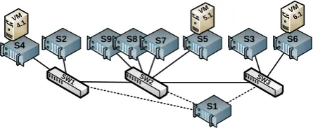
Figure 5: Network topology used in the experiment. Dashed links are used for monitoring, solid links for data traffic. ServerS1 is the experiment controller.
versity of Cambridge. The system consists of multiple dis-tributed components and is based on the SBUS/PIRATES (short SBUS) middleware.
In the case study, we consider two types of SBUS com-ponents: camera components and license plate recognition (LPR) components. The cameras are located in the city and take pictures of cars that are speeding or entering a paid zone. Each camera is connected to a respective SBUS com-ponent that sends the picture together with a time stamp to an LPR component. The LPR components are deployed in a data center due to their high consumption of computing resources. LPRs receive the pictures emitted by cameras and run a recognition algorithm to identify the license plate numbers of the observed vehicles.
5.2
Reference Models
Reference models serve as a baseline to evaluate the pre-diction accuracies of the generated predictive models. We consider two reference models in the evaluation. First, we consider the original SBUS implementation from the TIME-EACM project. Second, we consider the uperf benchmark [2] configured to mimic the traffic generated by the SBUS implementation and to abstract the application logic of the SBUS components (Camera, LPR) used in the case study. In [29], uperf was shown to correctly represent the traffic patterns of the SBUS implementation allowing the system to scale to picture generation frequencies that cannot be handled by the original SBUS implementation.
5.3
Hardware and Configuration
The system under study was deployed in a local data cen-ter consisting of nine servers and three switches. Each server is equipped with four 1GbpsEthernet ports. The switches are HP ProCurve 3500yl. The physical topology and the configuration of the network environment is depicted in Fig-ure 5. Server S1 is used to control the experiment and to acquire the monitoring data from switches using SNMP. Two servers,S2 andS3, are native (not virtualized). The nodes
S4–S6 are hosting VMs, whereasS8 hosts VMware Control Center andS9 is a storage.
5.4
Model Calibration
The DNI model describes the presented network, however, to be useful for performance prediction, it first needs to be annotated with performance-relevant information.
5.4.1
Network Structure
us-ing the values provided in the technical specifications of the respective devices. In such way, we describe all network interfaces of switches and physical hosts. The links them-selves are physical media and the only factor that influences their performance is the propagation delay, which is speci-fied as a tabulated value for the underlying network. Also the switching delays are specified in the technical documen-tation. Much more challenging is to calibrate other param-eters, like for example, speeds of virtual entities, protocol overheads, and traffic models.
5.4.2
Protocols
Information about protocol overheads is extracted from the operating system. Parameters like the MTU (Maximum Transmission Unit) and the length of a data unit header play an important role for calculating protocol overheads: every message is divided by the MTU value (to estimate the number of packets) and then the header overhead is added to each packet. The size of the message is then increased by the sum of packet overheads. ForDNI-to-QPN, this calcu-lation is done in the transformation; OMNeT++ simulates it internally, whereas mDNI-to-QPN ignores the protocol overheads.
5.4.3
Traffic Patterns
The traffic patterns are modeled manually on the proto-col level based on traffic monitoring tools or tcpdump traces. Silence intervals between sending consecutive messages are calculated manually and averaged over the duration of the entire experiment. In case of any parameter variability, a probability distribution can be constructed. Additionally, we verify if the intergeneration times configured in the soft-ware (e.g.,
”send a picture every 10ms”) match the times that are derived from the tcpdump. For our experiments, we describe this process, its consequences, and challenges in section 5.6.
5.4.4
Server Virtualization
Another challenging part is the extraction of the parame-ters that describe the virtual entities. In case of data trans-mission from one VM to another collocated VM, the data is in fact copied between memory cells. The exact path of the data and the overheads depend on the hypervisor type and the delays are difficult to estimate a priori. Addition-ally, the performance of the network bridge that is built-in in the hypervisor depends on the system load, which is not reflected in DNI since all model input parameters (e.g., re-source demands) are modeled as load-independent.
The values of the performance parameters describing vir-tual entities are finally estimated experimentally and mod-eled in a black-box manner. In this case study, we examine the performance of the hypervisor-emulated network by run-ning stress tests defined in uperf. The average bandwidth achieved in the tests is used directly to describe the speeds of the virtual network interfaces in VMs and in the hypervisor bridge.
5.5
Measurements
To obtain the baseline performance values, we measure the amount of the traffic flowing through the real network interfaces of all switches. We use the counters located in the switches to measure the number of bytes transmitted through each interface. We read the values of the
coun-ters through SNMP every second and calculate the aver-age throughput for that interval. ServerS1 makes measure-ments using an isolated VLAN. The experimental network was isolated from other networks (e.g., the Internet). During the measurements, all intergeneration times were modeled as exponentially distributed; confidence intervals are calculated for a significance level ofα= 0.05. In every experiment, we send predefined amount of pictures (5 000 for each camera) and execute the experiment 30 times for SBUS, uperf, and OMNeT++ and once for QPN (SimQPN cares internally about the required amount of repetitions).
5.6
Results
We evaluate the proposed approach in two scenarios. The goal of scenario 1 is to evaluate the accuracy of throughput prediction. We deploy the camera components and the LPR components and configure the communication between the components according to the following plan: S2→VM4.1, S2→VM5.1, S3→VM6.1, and S3→VM5.1. In this scenario, we increase the amount of transmitted pictures per second by decreasing the think time between sending consecutive pictures to: 100, 50, 35, 20, and 10ms respectively. We also measure the wall-clock times for every simulation and for the SBUS experiment. In scenario 2, we compare simula-tion durasimula-tions for growing traffic intensity and the increasing number of servers in the data center.
5.6.1
Prediction Accuracy
In the evaluation of the prediction accuracy, we measure the throughput on the switch ports (for the reference mod-els: SBUS and uperf) and compare them against the values predicted by the generated simulation models. In this ex-periment, we measure throughputs on selected switch inter-faces: S2→SW1, S3→SW3, and SW2→S5. In scenario 1, we expect the monitored throughputs to be equal on each inter-face. The variations may happen when the network capacity is saturated as the TCP protocol may divide the through-put unequally among the flows. The results are presented in Table 3.
Based on the gathered results, we observe the expected equalities in the measured and predicted throughputs for scenarios 1A–1D. By unsaturated network, the two refer-ence models performed similarly (max. 5.3% throughput variation relatively). For scenario 1E (saturated network), we observe wide confidence interval for the SBUS model. This phenomenon was observed in our previous workshop work [29] and is caused by software performance bottlenecks in the original SBUS implementation. For that scenario, we use uperf as the reference model. The predictions of the gen-erated models follow the measured trends with average rela-tive error of 7.4% for OMNeT++, 9.9% for the QPN(DNI), and 11.4% for the QPN(miniDNI).
OMNeT++. The OMNeT++ model predicted the through-put with the lowest average relative prediction error 7.4% (calculated as the relative difference between the mid points of confidence intervals). However, in scenario 1D, OMNeT++ reported the highest inaccuracy of 19% mispredicting the throughput maximally by 117 Mbps for the link SW2→S5. We have investigated the inaccuracy of the model and for-mulate the following observations and challenges.
multi-Table 3: Scenario 1A-E: measured and predicted throughput in mega-bits per second
Link SBUS uperf OMNeT QPN QPN
reference1 reference2 DNI DNI mDNI
lCI uCI lCI uCI lCI uCI avg. avg.
Scenario 1A (think time 100ms)
S2→SW1 205 216 211 219 199 224 202 202
SW2→S5 205 215 211 219 199 214 202 202
S3→SW3 204 215 210 220 200 223 202 202
Scenario 1B (think time 50ms)
S2→SW1 430 449 385 410 407 448 450 450
SW2→S5 431 447 390 403 404 437 450 450
S3→SW3 430 447 383 410 408 442 450 450
Scenario 1C (think time 35ms)
S2→SW1 541 562 496 539 471 530 578 578
SW2→S5 526 548 505 528 454 517 578 578
S3→SW3 524 551 495 538 419 484 578 578
Scenario 1D (think time 20ms)
S2→SW1 631 640 579 652 702 764 675 675
SW2→S5 639 648 583 640 689 752 675 675
S3→SW3 416 426 575 648 657 728 675 675
Scenario 1E (think time 10ms)
S2→SW1 686 941 882 941 914 942 978 1074
SW2→S5 482 506 884 939 883 909 978 1074
S3→SW3 615 941 882 941 914 942 978 1074
ple fine-grained parameters that influence the performance, however, we do not model the values of those parameters in DNI. OMNeT++ uses for simulation a larger set of param-eters than we are able to calculate in the transformation. The parameters that are not included in the DNI meta-model (e.g., TCP congestion algorithms, window size) are not transformed, and thus are set in OMNeT++ to their default values. To increase the prediction accuracy, a sim-ulator with finer granularity shall be used or the missing parameters should be provided manually.
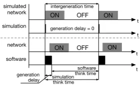
Second, the calibration of the traffic patterns (here we use the ON-OFF traffic pattern) is done manually based on the protocol level traces. Manual calibration procedures are er-ror prone and the erer-rors usually cumulate when the network is under high load. In scenario 1, the main challenge was the extraction of the think time value. We depict schematically this phenomenon in Figure 6. Although we set the think time in the software as predefined value, it does not mean, that on the protocol level the respective value remains the same. In many simulators (also in OMNeT++), the traf-fic generation process happens immediately, whereas in the software, the transmitted data must be copied between the respective memory cells and the respective mutexes need to be freed before asleepinstruction can be executed. The pre-cise modeling of the generation delay may be omitted by in-frequent data generations, however, by low think times this parameter has strong influence on the predicted values. The duration of the generation delay depends on the respective software implementation. In case of a single threaded imple-mentation (e.g., in case of SBUS), the generation delay may take significant time, for example: for 1MB message and a 1Gbit/s network interface, the generation of a message takes about 7ms. The precise calculation of the generation delay requires the available throughput to be known beforehand; this causes the fine model calibration challenging.
QPN.Both generated QPN models performed identically in low-load scenarios (1A–1D). The average prediction errors for theDNI QPN model are usually below 10% (with
max-ON
ON ON
simulated network
simulation
network
software
OFF
OFF ON generation delay = 0
t
t
t
t software
think time generation
delay simulationthink time intergeneration time
Figure 6: Differences between think times in simu-lation (upper part) and in the software (lower part).
imal error of 13.5% in scenario 1B), whereas forminiDNI QPN: 11.4% (maximum of 17.8% for scenario 1E).
The differences between the two QPN models appear first when the network gets saturated. In scenario 1E, the model generated from the miniDNI overestimates the measured throughput by about 160 Mbps reporting higher throughput than achievable in the practice. The reason for that is the level of abstraction applied in the generated QPN model— the protocol-related parameters are abstracted in the trans-formation. Additionally, the traffic calibration plays here an important role. Although the traffic patterns are not re-flected inminiDNI, theDNI2miniDNI transformation relies on the traffic patterns to aggregate the traffic information. Thus, errors caused by the imprecise DNI calibration prop-agate to the QPN model.
5.6.2
Simulation Time
Along with the prediction precision, we evaluated the per-formance of the generated simulation models, i.e., the time needed to solve them. Depending on the situation, a less pre-cise but quickly obtained result may be more valuable than precise but late predictions. During the execution of sce-nario 1, we measured the execution time of the experiments and the three generated simulation models. We examined the run durations in two scenarios: 2Aand 2B. First (2A), we varied the traffic intensity for the prediction accuracy scenario. Second (2B), we increased the size of the network by adding servers, whereas the traffic intensity was constant. The duration of simulations are measured using thetime command on a non-virtualized server with Intel Xeon E3-1230 CPU, 16GB RAM, and Ubuntu Linux 12.04. We com-pile OMNeT++ in the release mode (make MODE=release) and exclude the TCL library (NO TCL=1 ./configure). Sim-ulations are run in the command line mode (cmdenv). Run durations for OMNeT++ are estimated because of relatively long simulation times. First, we measure wall-clock time re-quired to simulate 30 seconds of the respective real time (OMNeT parameter: sim-time-limit). During this simula-tion period, we observe the
”simulation-seconds per second” parameter that describes the performance of the simulation. Then, we estimate the duration of the full simulation based on the real SBUS experiment duration and the measure-ments for 30 simulation-seconds. For selected simulation runs, we verify the estimations by simulating the complete experiment length. The verification shows, that the estima-tions are precise (up to 1% error).
sim-Table 4: Scenario 2A: model solution duration (in seconds) for growing traffic intensity
Think time
SBUS (real)
OMNeT 30s
OMNeT full
QPN DNI
QPN mDNI
100ms 1136 92 666 17 3
50ms 670 175 3908 31 3
35ms 528 234 4118 48 3
20ms 416 351 4867 73 3
10ms 348 519 6020 222 3
Simulation
duration
[s]
Traffic intensity (think time) [ms] OMNeT++ (30s)
DNI QPN miniDNI QPN
0 100 200 300 400 500
10 20 30 40 50 60 70 80 90 100
(a) Scenario 2A
Simulation
duration
[s]
Number of nodes OMNeT++ (30s)
DNI QPN miniDNI QPN
0 100 200 300 400 500 600 700 800 900
10 20 30 40 50 60 70 80 90 100
(b) Scenario 2B
Figure 7: Scenarios 2A and 2B: model solution du-ration (in seconds) for growing traffic intensity (2A) and network size (2B)
ulation models execute visibly slower than the QPNs—up to 100 minutes for 10msthink time. We observe exponen-tial growth of the simulation time for OMNeT++ andDNI QPN for growing traffic intensity. The miniDNI QPN model is insensitive to the traffic intensity and offers constant ulation time of 3 seconds. The exponential growth of sim-ulation duration for OMNeT++ and DNI QPN is caused by the increasing number of events/tokens in the simula-tion model. TheminiDNI QPN model abstracts the traffic patterns in the transformation and thus maintains constant number of tokens and constant simulation time.
Scenario 2B: Network Size. In this scenario, we assume a classical dumbbell topology with two directly connected switches and servers connected to them. We increase the number of servers connected to each switch while the traffic characteristics remain the same. Every node is set to trans-mit two 800KB pictures per second. The experiment is over when each node has finished the transmission of 5000 pic-tures. We generate 6 setups containing 5, 10, 20, 30, 40, and 50 nodes for each switch, i.e., 10, 20, 60, 80, and 100 nodes in total respectively. The simulation durations are presented in Table 5 and depicted in Figures 7a and 7b. Additionally, in the column
”Transf.”, we present the total time of the DNI model generation and the five model-to-model trans-formations. The source code of the transformations was not performance-optimized so the transformation duration can be further reduced.
In scenario 2B, we observe a linear growth of simulation time for OMNeT++ which is caused by the linear growth of the number of events in the simulation engine. This obser-vation confirms the results obtained by Weingartner et al. in [35]. Similar dependency can be observed forminiDNI QPN where the number of tokens grows linearly with respect to the number of nodes. The DNI QPN model experiences exponential growth of the simulation duration. Despite the linear nature of the OMNeT++ run duration, theDNI QPN outperforms the full length run of OMNeT++ by the factor
Table 5: Scenario 2B: transformation and model solution duration (in seconds) for growing network size
Nodes OMNeT
30s
OMNeT full
QPN DNI
QPN
mDNI Transf.
2×5 35 2953 21 5 25
2×10 65 5484 56 13 67
2×20 127 10716 183 36 149
2×30 195 16453 376 72 277
2×40 262 22106 630 122 446
2×50 334 28181 884 182 692
of 30. In scenario 2B, theminiDNI QPN model is solved on average 300 times faster than the respective full-length OMNeT++ simulation;miniDNI QPN requires four times less simulation time than the respectiveDNI QPN model.
6.
CONCLUSIONS AND FUTURE WORK
In this paper, we show that abstraction of selected details in network performance models can lead to only minor pre-diction accuracy degradation (up to 4% on average) but can accelerate the performance analysis by factor of 300. We stress, that maximized accuracy of performance prediction requires highly-detailed, protocol-level modeling formalisms. In our approach, we accept lower prediction accuracy by pro-viding technology independent generic modeling formalism. Despite the introduced abstractions in theDNI meta-model and fully automatic process of predictive model generation, we obtain good throughput prediction accuracy with maxi-mal prediction error up to 18%.
Using theDNI meta-model and the proposed model-to-model transformations, we automatically obtain simulation models with different modeling granularity. The generated simulation models can be flexibly used according to the sit-uation: less analysis overhead and less prediction accuracy or longer simulations but more accurate predictions. Our approach requires a single inputDNI model and offers mul-tiple predictive models without requiring any expertise in each of them. Non-experts can clearly benefit from our ap-proach because they learn only one modeling formalism but receive multiple automatically generated models.
Obtaining good prediction accuracy requires careful model calibration. We formulate the technical challenges that need to be considered during the calibration process. For exam-ple, imprecise modeling of network traffic patterns, can vis-ibly influence the predicted throughput values. To precisely tune the model parameters, a low-level trace-based calibra-tion is recommended. We plan to support this process in our future work by providing tools and methods for auto-mated or semi-autoauto-mated calibration. Additionally, we plan to evaluate theDNI meta-model in SDN scenarios for data center networks. Furthermore, we plan to add support for additional performance metrics like transmission delay and network latency.
7.
REFERENCES
[1] SDL combined with UML. ITU-T Z.109, 2000. [2] uperf A network performance tool, 2012. [3] OMG’s Meta-ObjectFacility, 2014.
InProceedings of the 5th IEEE Consumer Communications and Networking Conference (CCNC), Las Vegas, 2008. [5] S. Balsamo, A. di Marco, P. Inverardi, and M. Simeoni.
Model-based performance prediction in software
development: a survey.Software Engineering, IEEE
Transactions on, 30(5):295–310, 2004.
[6] S. Becker, H. Koziolek, and R. Reussner. The Palladio component model for model-driven performance prediction.
Journal of Systems and Software, 82(1):3–22, 2009. [7] S. Bernardi and J. Merseguer. Performance evaluation of
UML design with Stochastic Well-formed Nets.Journal of
Systems and Software, 80(11):1843–1865, 2007. [8] J. Britton and A. deVos. Cim-based standards and cim
evolution.IEEE Transactions on Power Systems,
20(2):758–764, May 2005.
[9] F. Brosig, N. Huber, and S. Kounev. Architecture-Level Software Performance Abstractions for Online Performance
Prediction.Elsevier Science of Computer Programming
Journal (SciCo), 2013.
[10] V. Cortellessa, P. Pierini, R. Spalazzese, and A. Vianale. Moses: Modeling software and platform architecture in uml 2 for simulation-based performance analysis. In S. Becker,
F. Plasil, and R. Reussner, editors,Quality of Software
Architectures. Models and Architectures, volume 5281 of
Lecture Notes in Computer Science, pages 86–102. Springer Berlin Heidelberg, 2008.
[11] N. de Wet and P. Kritzinger. Using UML models for the
performance analysis of network systems.Comput. Netw.,
49(5):627–642, 2005.
[12] W. E. Denzel, J. Li, P. Walker, and Y. Jin. A framework for end-to-end simulation of high-performance computing
systems. InProceedings of the 1st International Conference
on Simulation Tools and Techniques for Communications, Networks and Systems & Workshops, Simutools, pages 21:1–21:10, 2008.
[13] I. Dietrich, F. Dressler, V. Schmitt, and R. German. SYNTONY: network protocol simulation based on
standard-conform UML2 models. InProc. of the
ValueTools ’07, pages 21:1–21:11, 2007.
[14] Q. Duan. Modeling and performance analysis on network virtualization for composite network-cloud service
provisioning. InServices (SERVICES), 2011 IEEE World
Congress on, pages 548–555, July 2011.
[15] A. J. Field, U. Harder, and P. G. Harrison. Network Traffic
Behaviour in Switched Ethernet Systems. InMASCOTS
2002, 10th IEEE International Symposium on Modeling, Analysis, and Simulation of Computer and
Telecommunications Systems, pages 32–42, October 2002.
[16] P. G. Harrison and N. M. Patel.Performance Modelling of
Communication Networks and Computer Architectures. Addison-Wesley, 1993.
[17] N. Huber, M. von Quast, M. Hauck, and S. Kounev. Evaluating and Modeling Virtualization Performance
Overhead for Cloud Environments. InProc. of the 1st Int.
Conf. on Cloud Computing and Services Science, pages 563–573, 2011.
[18] I. Kaj and J. Ols´en. Throughput modeling and simulation
for single connection tcp-tahoe. In J. M. de Souza, N. L.
da Fonseca, and E. A. de Souza e Silva, editors,Teletraffic
Engineering in the Internet Era, volume 4 ofTeletraffic Science and Engineering, pages 705–718. Elsevier, 2001. [19] D. Kolovos, R. Paige, and F. A. Polack. The Epsilon
Transformation Language. InTheory and Practice of Model
Transformations, vol. 5063 of LNCS, pages 46–60. Springer, 2008.
[20] S. Kounev, K. Bender, F. Brosig, N. Huber, and R. Okamoto. Automated Simulation-Based Capacity
Planning for Enterprise Data Fabrics. In4th International
ICST Conference on Simulation Tools and Techniques, pages 27–36, 2011.
[21] L. Kristensen and K. Jensen. Specification and validation of an edge router discovery protocol for mobile ad hoc
networks. InIntegration of Software Specification
Techniques for Applications in Engineering, pages 248–269. 2004.
[22] N. McKeown, T. Anderson, H. Balakrishnan, G. Parulkar, L. Peterson, J. Rexford, S. Shenker, and J. Turner. Openflow: enabling innovation in campus networks.
SIGCOMM Comput. Commun. Rev., 38(2):69–74, 2008. [23] Object Management Group (OMG). UML Profile for
Modeling and Analysis of Real-Time and Embedded systems (MARTE), May 2006.
[24] A. Prakash, Z. Theisz, and R. Chaparadza. Formal methods for modeling, refining and verifying autonomic
components of computer networks. InTransactions on
Computational Science XV, pages 1–48. Springer, 2012. [25] R. Puigjaner. Performance modelling of computer
networks. InProc. of the 2003 IFIP/ACM Latin America
conf. on Towards a Latin American agenda for network research, LANC ’03, pages 106–123, New York, NY, USA, 2003. ACM.
[26] G. Riley and T. Henderson. The ns-3 network simulator. In
K. Wehrle, M. G¨unes, and J. Gross, editors,Modeling and
Tools for Network Simulation, pages 15–34. Springer Berlin Heidelberg, 2010.
[27] P. Rygielski and S. Kounev. Data Center Network
Throughput Analysis using Queueing Petri Nets. In34th
IEEE International Conference on Distributed Computing Systems Workshops. 4th International Workshop on Data Center Performance, (DCPerf 2014), pages 100–105, 2014. [28] P. Rygielski and S. Kounev. Descartes Network
Infrastructures (DNI) Manual: Meta-models, Transformations, Examples. Technical Report, 2014. [29] P. Rygielski, S. Kounev, and S. Zschaler. Model-Based
Throughput Prediction in Data Center Networks. InProc.
of the 2nd IEEE Int. Workshop on Measurements and Networking, pages 167–172, 2013.
[30] P. Rygielski, S. Zschaler, and S. Kounev. A metamodel for Performance Modeling of Dynamic Virtualized Network
Infrastructures (Work-in-progess paper). InProc. of the 4th
ACM/SPEC Int. Conf. on Performance Engineering, pages 327–330. ACM, 2013.
[31] A. Varga. The OMNeT++ discrete event simulation
system. InProc. of the European Simulation
Multi-conference, pages 319–324, 2001.
[32] J. G. von Kistowski, N. R. Herbst, and S. Kounev. LIMBO: A Tool For Modeling Variable Load Intensities. In
Proceedings of the 5th ACM/SPEC International Conference on Performance Engineering (ICPE), pages 225–226. ACM, 2014.
[33] G. Wang and T. Ng. The impact of virtualization on network performance of amazon ec2 data center. In
Proceedings of IEEE INFOCOM, pages 1–9, 2010.
[34] K. Wehrle, M. G¨unes, and J. Gross, editors.Modeling and
Tools for Network Simulation. Springer, 2010. [35] E. Weingartner, H. vom Lehn, and K. Wehrle. A
performance comparison of recent network simulators. In
IEEE International Conference on Communications, pages 1–5, 2009.
[36] M. Woodside, D. C. Petriu, D. B. Petriu, H. Shen, T. Israr, and J. Merseguer. Performance by unified model analysis
(puma). InProceedings of the 5th International Workshop
on Software and Performance, pages 1–12. ACM, 2005. [37] D. A. Zaitsev and T. R. Shmeleva. A Parametric Colored
Petri Net Model of a Switched Network.Int. J.