http://www.sciencepublishinggroup.com/j/ajsea doi: 10.11648/j.ajsea.20170603.11
ISSN: 2327-2473 (Print); ISSN: 2327-249X (Online)
Comparative Study of Least Square Methods for Tuning
Erceg Pathloss Model
Nnadi Nathaniel Chimaobi
1, Charles Chukwuemeka Nnadi
1, Amaechi Justice Nzegwu
21Department of Electrical/Electronic Engineering Imo State Polytechnic, Umuagwo, Owerri, Nigeria 2
Department of Science Laboratory Technology Imo State Polytechnic, Umuagwo, Owerri, Nigeria
Email address:
[email protected] (N. N. Chimaobi)
To cite this article:
Nnadi Nathaniel Chimaobi, Charles Chukwuemeka Nnadi, Amaechi Justice Nzegwu. Comparative Study of Least Square Methods for Tuning Erceg Pathloss Model. American Journal of Software Engineering and Applications. Vol. 6, No. 3, 2017, pp. 61-66.
doi: 10.11648/j.ajsea.20170603.11
Received: January 8, 2017; Accepted: January 18, 2017; Published: June 12, 2017
Abstract:
In this paper, a study of two least square error approaches for optimizing Erceg pathloss model is presented. The first approach is implemented by the addition of the root mean square error (RMSE) if the sum of prediction errors is positive otherwise, the RMSE is subtracted from the pathloss predicted by the original Erceg model. In the second method, the composition function of the residue is used to generate the model correction factor that is added to the original Erceg model pathloss prediction. The study is based on field measurement carried out in a suburban area for a GSM network in the 800 MHz frequency band. The results show that the untuned Erceg model has RMSE of 59.27384 dB and prediction accuracy of 59.57243%. On the other hand, the pathloss predicted by the RMSE tuned Erceg model has RMSE of 4.495422dB and prediction accuracy of 97.28188% and the pathloss predicted by the composition function tuned Erceg model has RME of 2.177523 dB and prediction accuracy of 98.7253%. In any case, the two methods are effective in minimizing the error to within the acceptable value of less than 7 dB. However, the composition function approach has better pathloss prediction performance with smaller RMSE and higher prediction accuracy than the RMSE-based approach.Keywords:
Pathloss, Erceg Model, Least Square Method, Propagation Model, Model Tuning, Composition Function Of Residue1. Introduction
In wireless network planning, pathloss are usually used in link budgeting and in the estimation of network coverage area [1-5]. Mostly, network planners find it easier to use pathloss models to estimate the pathloss that can be experienced by the signal in any given area [6-10]. In this wise, empirical pathloss models are usually the first option in view of their simplicity and quite acceptable pathloss prediction capability [11-16].
However, for more accurate estimation of pathloss in any given terrain, empirical pathloss models are usually subjected to empirical prediction performance evaluation and further or optimization with respect to field measured pathloss values. In most published literatures, the least square error optimization approach is mostly used [17-21]. There are different approaches to implement the least square optimization of
pathloss model. The simplest approach is to generate the root mean square error (RMSE) from the measured and the models predicted pathloss and then add or subtract the RMSE from the pathloss predicted at each there is measurement pathloss. Other method is the adjustment of some coefficients in the original pathloss model so as to minimize the error. yet, another approach if to use function of function approach to estimate the prediction error as a function of the predicted pathloss.
2. Theoretical Background
2.1. Erceg Path Loss Model
The Erceg model has been chosen by IEEE 802.16 as
reference propagation model for WiMAX system evaluation [22-26]. This model can be applied in three different environments, Type A, B and C. By using this model the total attenuation ( ) for outdoor is given by [27]:
( ) = + 10 log + + + ! > ! (1)
Where,
f = The frequency in MHz
d = The distance between AP and CPE antennas in meters
! =100m
= The correction for receiving the antenna height in meters
= The path loss exponent
= The correction for frequency in MHz
S = The correction for shadowing in dB and its value is between 8.2 and 10.6 dB at the presence of trees and other clutters on the propagation path
The parameter A is defined as:
= 20 log $%ʎ (2)
and the path loss exponent is given by:
= ' + ((ℎ*) + +, (3)
Where, the parameter ℎ* is the base station antenna height in meters. This is between 10 m and 80 m. The constants a, b and c depend upon the types of terrain, that are given in Table 1. The value of parameter is 2 for free space propagation in an urban area, 3 < < 5 for urban none line of sight (NLOS) environment, and > 5 for indoor propagation.
Table 1. The Erceg Parameters.
Parameters Type A Type B Type C
! 100m 100m 100m
a 4.6 4.0 3.6
b 0.0075 01 0.0065 01 0.0050 01
c 12.6m 17.1m 20.0m
The frequency correction factor, Xf and the correction for receiver antenna height, Xh are expressed as:
= 6 log 3 (4)
= −10.8 log 6
3 for terrain type A and B (5)
= −20.8 log 6
3 for terrain type C (6)
Where, f is the operating frequency in MHz, and ℎD is the receiver antenna height in meter.
Type A is associated with maximum path loss and is appropriate for hilly terrain with moderate to heavy foliage densities.
Type B is characterized with either mostly flat terrains with moderate to heavy tree densities or hilly terrains with light tree densities.
Type C is associated with minimum path loss and applies to flat terrain with light tree densities.
2.2. Data Collection and Processing
The Received Signal Strength (RSS) and spatial data (longitude and latitude) dataset are then collected along a rout selected for the study. Samsung Galaxy S4 mobile phone with Cellmapper android application installed is used to capture and store the dataset (RSS and spatial datasets) as CSV file. The RSS is converted to the measured pathloss (PLG (HI)) using the formula [13-15]:
D ( ) = PBTS + GBTS + GMS – LFC – LAB – LCF – RSS (dBm) (7)
where
PLG (HI) is the measured pathloss for each measurement location at a distance d ( km)
RSS is the mean Received Signal Strength in dBm, that is, the measured received signal strength.
PBTS is the Transmitter Power (dBm), GBTS is the
Transmitter Antenna Gain (dBi), GMS is the receiver antenna
gain (dBi), LFC is the feeder cable and connector loss (dB),
LAB is the Antenna Body Loss (dB) and LCF is the Combiner
and Filter Loss (dB).
The values of these parameters are given as [13] as: PBTS =
40 W = 46 dBm, GBTS = 18.15 dBi, GMS = 0 dBi, LFC = 3 dB,
LAB = 3 dB, LCF = 4.7 dB. Hence,
D ( ) = 53.5 (dBm).– RSS (dBm) (8) Again, the Haversine formula in Eq 9 is used to computer the distances (d) between each measurement point and the base station as follows;
! = 2 NOsin PQRS1PQRT 3
3
+ cos( V ) cos( V3) sin PWX S1PWX3 T 3 S
Y (9)
LAT in Radians = (Z[\ ]^ _`ab``c ∗ e. $3)f (10)
LONG in Radians = (Zghi ]^ _`ab``c ∗ e. $3)f (11)
Where
LAT1 and LAT2 are the latitude of the coordinates of point1 and point 2 respectively
LONG1 and LONG2 are the longitude of the coordinates of point1 and point 2 respectively
d = the distance between the two coordinates
2.3. Performance Analysis of the Models
These statistical performance measures or goodness of fit measures for the Erceg model are defined as follows:
i) The Root Mean Square Error (RMSE) is calculated as follows:
MSE = Om S no∑w z nw z q (Drstuvr ) (w)− (xvr w+yr ) (w) q3{| (12)
ii) Then, the Prediction Accuracy (PA, %) based on mean absolute percentage deviation (MAPD) or Mean Absolute Percentage Error (MAPE) is calculated as follows:
PA = }1 −n ~∑ •q€P(6•‚ƒ„…•†) (‡)1€P(ˆ…•†‡‰Š•†) (‡) q
€P(6•‚ƒ„…•†)(‡) •
wzn
wz ‹Œ * 100% (13)
2.4. Model Optimization Process
The parameters of the Erceg pathloss model were adjusted (optimized) using two different least square methods as follows;
1) First, the residual (or error, e) between measured pathloss, D ( ) and the Erceg model predicted pathloss D ( ) is calculated for each location point, i.
• (w) = D ( ) (w) - D ( ) (w) (14)
2) Second, the RMSE is calculated based along with sum of errors, that is ∑ Ž•wzn wz (w) •.
3) Thirdly, if ∑ Ž•wzn wz (w) • < 0 then the optimised model is obtained by subtracting RMSE from each D ( ) (w) otherwise, if ∑ Ž•wzn wz (w) • ≥ 0 the optimised model is obtained by adding RMSE to each D ( ) (w).
4) Fourtly, if ∑ Ž•wzn wz (w) • < 0 then the optimised model is obtained by subtracting RMSE from each D ( ) (w) otherwise, if ∑ Ž•wzn wz (w) • ≥ 0 the optimised model is obtained by adding RMSE to each D ( ) (w).
D ( ) (w) = D ( ) (w) + • (w) (15) Where • (w) is estimated from a composite function,
•Ž D ( ) (w)• defined as follows;
•Ž D ( ) (w)• = K1 ( D ( ) (w)) +K2
K1 and K2 are the tuning coefficients for the composition of function of residual given as Ž D ( ) (w)•. Essentially,
•Ž D ( ) (w)• is a function the predicts the residue (that is, the prediction error, • (w) ) based on the pathloss predicted by the untuned Erceg model. Furthermore, • (w) ≈
•Ž D ( ) (w)•, then;
D ( ) (w) = D ( ) (w) +K1 ( D ( ) (w)) +K2 =(16)
The composite function tune Erceg model is therefore given as ‘R ( ) (w) where
‘R ( ) (w)= D ( ) (w) +K1 ( D ( ) (w)) +K2 (17)
3. Results and Discussions
The field measured distance, received signal strength (RSSI) and pathloss (PLm) are given in Table 2. The measured pathloss (PLm) is obtain by applying link budget equation, D ( ) = 53.5 (dBm) – RSS (dBm) to each of the measured received signal strength. Furthermore, Haversine formula is used to obtain the distance between the GSM base station and each of the measurement point, where the longitude 1 and latitude 1 are that of the GSM base station while longitude 2 and latitude 2 are for each of the measurement points.
Figure 1 shows the radial graph of measured pathloss in dB versus distance in meters. The measure pathloss values are from 134.5 dB at a distance of 773m from the GSM base station to a pathloss value of 152.5dB at a distance of 1012 m from the GSM base station.
Table 2. The Field Measured Distance, Received Signal Strength (RSS) and Field Measured Path Loss (PLm).
S/N d (km) RSS (dB) Field Measured Path Loss (dB) S/N d (km) RSS (dB) Field Measured Path Loss (dB)
1 0.772603 -81 134.5 15 0.9 -97 150.5
2 0.804 -85 138.5 16 0.911 -97 150.5
3 0.82 -85 138.5 17 0.912 -97 150.5
4 0.83 -85 138.5 18 0.913 -97 150.5
5 0.84 -85 138.5 19 0.92 -97 150.5
6 0.848 -85 138.5 20 0.922 -97 150.5
7 0.857 -91 144.5 21 0.93 -97 150.5
8 0.863 -91 144.5 22 0.936 -97 150.5
9 0.863 -91 144.5 23 0.951 -97 150.5
10 0.871 -91 144.5 24 0.965 -97 150.5
11 0.878 -91 144.5 25 0.984 -97 150.5
12 0.89 -91 144.5 26 1.001 -97 150.5
13 0.894 -91 144.5 27 1.012 -99 152.5
14 0.9 -91 144.5
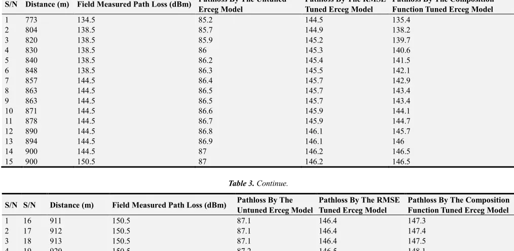
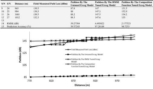
Table 3 and figure 1 show the field measure pathloss and the pathloss predicted by the untuned Erceg model, the pathloss predicted by the RMSE tuned Erceg model and the pathloss predicted by the composition function tuned Erceg model.
accuracy of 97.28188%. and the pathloss predicted by the composition function tuned Erceg model has RME of 2.177523 dB and prediction accuracy of 98.7253%. Given that
RMSE 59.27384, for the untuned Erceg model then the composition function is obtained as;
•Ž D w• = 5.306988273 ( D w) - 401.9577187 (18)
So,
‘R w D w 5.306988273 ( D w ) -
401.9577187 (19)
Figure 1. The radial graph of measured pathloss in dB versus distance in meters.
Table 3. The field measure pathloss and the pathloss predicted by the untuned and the tuned Erceg models.
S/N Distance (m) Field Measured Path Loss (dBm) Pathloss By The Untuned Erceg Model
Pathloss By The RMSE Tuned Erceg Model
Pathloss By The Composition Function Tuned Erceg Model
1 773 134.5 85.2 144.5 135.4
2 804 138.5 85.7 144.9 138.2
3 820 138.5 85.9 145.2 139.7
4 830 138.5 86 145.3 140.6
5 840 138.5 86.2 145.4 141.5
6 848 138.5 86.3 145.5 142.1
7 857 144.5 86.4 145.7 142.9
8 863 144.5 86.5 145.7 143.4
9 863 144.5 86.5 145.7 143.4
10 871 144.5 86.6 145.9 144.1
11 878 144.5 86.7 145.9 144.7
12 890 144.5 86.8 146.1 145.7
13 894 144.5 86.9 146.1 146
14 900 144.5 87 146.2 146.5
15 900 150.5 87 146.2 146.5
Table 3. Continue.
S/N S/N Distance (m) Field Measured Path Loss (dBm) Pathloss By The Untuned Erceg Model
Pathloss By The RMSE Tuned Erceg Model
Pathloss By The Composition Function Tuned Erceg Model
1 16 911 150.5 87.1 146.4 147.3
2 17 912 150.5 87.1 146.4 147.4
3 18 913 150.5 87.1 146.4 147.5
4 19 920 150.5 87.2 146.5 148.1
5 20 922 150.5 87.2 146.5 148.2
6 21 930 150.5 87.3 146.6 148.9
7 22 936 150.5 87.4 146.7 149.3
S/N S/N Distance (m) Field Measured Path Loss (dBm) Pathloss By The Untuned Erceg Model
Pathloss By The RMSE Tuned Erceg Model
Pathloss By The Composition Function Tuned Erceg Model
9 24 965 150.5 87.8 147 151.5
10 25 984 150.5 88 147.3 152.9
11 26 1001 150.5 88.2 147.5 154.2
12 27 1012 152.5 88.3 147.6 155
13
14 RMSE (dB) 59.27384 4.495422 2.177523
15 Prediction Accuracy (%) 59.57243 97.28188 98.7253
Figure 2. The field measure pathloss and the pathloss predicted by the untuned and the tuned Erceg model.
4. Conclusion
In this paper, comparative study of two least square error approaches for optimizing Erceg pathloss model is presented. Both methods are by adding or subtracting a model correction factor. In the first model tuning approach the correction factor is the root mean square error (RMSE). It is implemented is the addition or subtraction of the RMSE based on whether the sum of errors is positive or negative. In the second method the correction factor is the composition function of the residue (that is function of the prediction error of the the original Erceg model). It is implemented by adding the composition function to the pathloss predicted by the Erceg model. The study is based on field measurement carried out in a suburban area for a GSM network in the 800MHz frequency band. The results show that the composition function approach has better pathloss prediction performance with smaller RMSE and higher prediction accuracy than the RMSE-based approach.
References
[1] Sharma, P. K., & Singh, R. K. (2012). Cell coverage area and link budget calculations in GSM system. International Journal of Modern Engineering Research (IJMER) vol, 2, 170-176.
[2] Kim, H. (2015) Wireless Communications Systems Design and Considerations. Wireless Communications Systems Design, 349-378.
[3] Isabona, J., & Obahiagbon, K. (2014). RF Propagation Measurement and Modelling to Support Adept Planning of Outdoor Wireless Local Area Networks in 2.4 GHz Band.
American Journal of Engineering Research (AJER) Volume-03, Issue-01, pp-258-267.
[4] Hamid, N. I. B., Kawser, M. T., & Hoque, M. A. (2012). Coverage and capacity analysis of LTE radio network planning considering Dhaka city. International Journal of Computer Applications, 46 (15), 49-56.
[5] Al Mahmud, M. R. (2009). Analysis and planning microwave link to established efficient wireless communications (Doctoral dissertation, Blekinge Institute of Technology).
[6] Luiz, T. A., Freitas, A. R., & Guimarães, F. G. (2015, July). A New Perspective on Channel Allocation in WLAN: Considering the Total Marginal Utility of the Connections for the Users. In Proceedings of the 2015 Annual Conference on Genetic and Evolutionary Computation (pp. 879-886). ACM.
[7] Sulyman, A. I., Nassar, A. T., Samimi, M. K., Maccartney, G. R., Rappaport, T. S., & Alsanie, A. (2014). Radio propagation path loss models for 5G cellular networks in the 28 GHz and 38 GHz millimeter-wave bands. IEEE Communications Magazine, 52 (9), 78-86.
[8] Sotiroudis, S. P., & Siakavara, K. (2015). Mobile radio propagation path loss prediction using artificial neural networks with optimal input information for urban environments. AEU-International Journal of Electronics and Communications, 69 (10), 1453-1463.
[9] Liechty, L. C. (2007). Path loss measurements and model analysis of a 2.4 GHz wireless network in an outdoor environment (Doctoral dissertation, Georgia Institute of Technology).
[11] Gustafson, C., Abbas, T., Bolin, D., & Tufvesson, F. (2015). Statistical modeling and estimation of censored pathloss data. IEEE Wireless Communications Letters, 4 (5), 569-572.
[12] Faruk, N., Ayeni, A., & Adediran, Y. A. (2013). On the study of empirical path loss models for accurate prediction of TV signal for secondary users. Progress In Electromagnetics Research B, 49, 155-176.
[13] Abhayawardhana, V. S., Wassell, I. J., Crosby, D., Sellars, M. P., & Brown, M. G. (2005, May). Comparison of empirical propagation path loss models for fixed wireless access systems. In 2005 IEEE 61st Vehicular Technology Conference (Vol. 1, pp. 73-77). IEEE.
[14] Popoola, S. I., & Oseni, O. F. (2014). Empirical Path Loss Models for GSM Network Deployment in Makurdi, Nigeria. International Refereed Journal of Engineering and Science (IRJES), 3 (6), 85-94.
[15] Akinwole, B. O. H., & Biebuma, J. J. (2013). Comparative Analysis of Empirical Path Loss Model For Cellular Transmission In Rivers State. Jurnal Ilmiah Electrical/Electronic Engineering, 2.
[16] Costa, J. C. (2008). Analysis and optimization of empirical path Loss models and shadowing effects for the Tampa Bay Area in the 2.6 GHz Band.
[17] Udofia, K. M., Friday, N., & Jimoh, A. J. (2016). Okumura-Hata Propagation Model Tuning Through Composite Function of Prediction Residual. Mathematical and Software Engineering, 2 (2), 93-104.
[18] Yin, X., Cai, X., Cheng, X., Chen, J., & Tian, M. (2015). Empirical Geometry-Based Random-Cluster Model for High-Speed-Train Channels in UMTS Networks. IEEE Transactions on Intelligent Transportation Systems, 16 (5), 2850-2861.
[19] Benedičič, L., Pesko, M., Javornik, T., & Korošec, P. (2014). A metaheuristic approach for propagation-model tuning in LTE networks. Informatica, 38 (3).
[20] Bhuvaneshwari, A., Hemalatha, R., & Satyasavithri, T. (2013, October). Statistical tuning of the best suited prediction model for measurements made in Hyderabad city of Southern India. In Proceedings of the world congress on engineering and computer science (Vol. 2, pp. 23-25).
[21] Mousa, Allam, et al. "Optimizing Outdoor Propagation Model based on Measurements for Multiple RF Cell." International Journal of Computer Applications 60.5 (2012).
[22] Udaykumar, R. Y. (2014, May). Performance investigation of mobile WiMAX protocol for aggregator and electrical vehicle communication in Vehicle-to-Grid (V2G). In Electrical and Computer Engineering (CCECE), 2014 IEEE 27th Canadian Conference on (pp. 1-6). IEEE.
[23] Zhang, X., & Andrews, J. G. (2015). Downlink cellular network analysis with multi-slope path loss models. IEEE Transactions on Communications, 63 (5), 1881-1894.
[24] Jadhav, A. N., & Kale, S. S. (2014). Suburban Area Path loss Propagation Prediction and Optimization Using Hata Model at 2375 MHz. International Journal of Advanced Research in Computer and Communication Engineering, 3 (1), 5004-5008.
[25] Alam, D., & Khan, R. H. (2013). Comparative study of path loss models of WiMAX at 2.5 GHz frequency band. International Journal of Future Generation Communication and Networking, 6 (2), 11-24.
[26] Imperatore, P., Salvadori, E., & Chlamtac, I. (2007, May). Path loss measurements at 3.5 GHz: a trial test WiMAX based in rural environment. In Testbeds and Research Infrastructure for the Development of Networks and Communities, 2007. TridentCom 2007. 3rd International Conference on (pp. 1-8). IEEE.