ISSN 2307-4531
http://gssrr.org/index.php?journal=InternationalJournalOfComputer&page=index
Minimization of Active Power Loss and Voltage
Profile Fortification by Using Differential Evolution –
Harmony Search Algorithm
K. Lenin
a*, Bhumanapally Ravindhranath Reddy
b, M. Surya
Kalavathi
ca,b,c
Jawaharlal Nehru Technological University Kukatpally, Hyderabad 500 085, India. a
Abstract
This paper presents DEHS (Differential Evolution-harmony Search) algorithm for solving the
multi-objective reactive power dispatch problem .Harmony Search is a new heuristic algorithm, which
mimics the procedure of a music player to search for an ideal state of harmony in music playing.
Harmony Search can autonomously mull over each component variable in a vector while it generates a
new vector. These features augment the flexibility of the Harmony Search algorithm and produce better
solutions and overcome the disadvantage of Differential Evolution. Improved Differential Evolution
method based on the Harmony Search Scheme, which we named it DEHS (Differential
Evolution-harmony Search). The DEHS method has two behaviors. On the one hand, DEHS has the flexibility. It
can adjust the values lightly in order to get a better global value for optimization. On the other hand,
DEHS can greatly boost the population’s diversity. It not only uses the DE’s strategies to search for
global optimal results, but also utilize HS’s tricks that generate a new vector by selecting the
components of different vectors randomly in the harmony memory and its outside. In order to evaluate
the proposed algorithm, it has been tested on IEEE 30 bus system and compared to other algorithms.
Key words: Modal analysis, optimal reactive power, Transmission loss, differential evolution, harmony.
--- * Corresponding author.
E-mail address: [email protected].
1. Introduction
Optimal reactive power dispatch problem is one of the complex optimization problems in power
system. The sources of the reactive power are the generators, synchronous condensers, capacitors,
static compensators and tap changing transformers. Here the reactive power dispatch problem involves
best operation of the existing generator bus voltage magnitudes, transformer tap setting and the output
of reactive power sources so as to minimize the real power loss and to boost the voltage stability of the
system. Various arithmetical techniques have been adopted to solve this optimal reactive power
dispatch problem. These include the gradient method [1-2], Newton method [3] and linear
programming [4-7].The gradient and Newton methods experience from the difficulty in handling
inequality constraints. To apply linear programming, the input- output function is to be expressed as a
set of linear functions which may lead to loss of accurateness. Newly Global Optimization techniques
such as genetic algorithms have been planned to solve the reactive power flow problem [8, 9]. To boost
the voltage stability, voltage magnitudes alone will not be a reliable indicator of how far an operating
point is from the collapse point [10]. The reactive power support and voltage problems are intrinsically
related. Hence, this paper formulates the reactive power dispatch as a multi-objective optimization
problem with loss minimization and maximization of static voltage stability margin (SVSM) as the
objectives. Global optimization has received extensive research attention, and a great number of
methods have been applied to solve this problem. Evolutionary algorithm is a heuristic approach for
minimizing possibly nonlinear and non-differentiable continuous space functions. For many decades,
evolutionary algorithms range from the first algorithm Genetic Algorithm (GA) [11] to Evolutionary
Strategies (ES) [12], Genetic Programming (GP) [13], Evolutionary Programming (EP) [14],
Differential Evolution (DE) [15], and other methods, such as Simulated Annealing (SA) [16], Particle
Swarm Optimizer (PSO) [17, 18], and Neural Networks [19]. All of these have been successfully
applied to a wide range of optimization problems, such as, image processing, pattern recognition,
scheduling, engineering design, and others [20]. DE algorithm as a novel version of GA is a
population-based stochastic direct search method for global optimization. Unlike GA that uses binary
coding to represent problem parameters, DE uses real valued parameters, which is easily applied to
experimental minimization where the cost value is derived from a physical experiment rather than a
computer simulation. DE has four advantages: ability to handle non-differentiable, nonlinear and
multi-modal cost functions; ability to parallel cope with computation intensive cost functions; ease of use;
and good convergence properties. It has been successfully applied to various benchmark and real-world
problems, including a travelling salesman problem [21], design centring [22], digital filter design [21,
23], and noisy objection functions [24], and so on. Harmony Search (HS) is a new heuristic algorithm
mimics the improvisation of music players, which was proposed by Geem [25]. HS is optimization
algorithms that seek a best state (global optimum-minimum cost or maximum benefit or efficiency)
determined by objective function assessment. It has been successfully used into various benchmark and
real-world problems, includes a travelling salesman problem [26], parameter optimization of river
flood model [27], design of pipeline network [28, 29], and design of truss structures [30]. In this paper,
we propose an improved DE combined with HS named DEHS, not only uses the DE’s strategies to
search for global optimal results, and utilize HS’s tricks that generate a new vector by selecting the
components of different vectors randomly in the harmony memory and its outside, but also uses the
pitch adjustment method to adjust the variables left or right in population of one generation. Our
algorithm is more flexible and greatly enhancements population’s diversity, which totally different
from Liao [31] proposed MDE-IHS method, which use the current Number of Function Evaluations
(NFE) to replace the parameter t in improvisation step [32-33]. As a result, DEHS avoided the optimal
function falling into local minimal. The proposed algorithm DEHS been evaluated in standard IEEE 30
bus test system & the results analysis shows that our proposed approach outperforms all approaches
investigated in this paper.
2. Voltage Stability Evaluation
2.1.Modal analysis for voltage stability evaluation
Modal analysis is one of the methods for voltage stability enhancement in power systems. The
linearized steady state system power flow equations are given by.
�∆∆QP�=�JJpθ Jpv
qθ JQV � (1)
Where
ΔP = Incremental change in bus real power.
ΔQ = Incremental change in bus reactive
Power injection
Δθ = incremental change in bus voltage angle.
ΔV = Incremental change in bus voltage Magnitude
Jpθ , J PV , J Qθ , J QV jacobian matrix are the sub-matrixes of the System voltage stability is
affected by both P and Q. However at each operating point we keep P constant and evaluate
voltage stability by considering incremental relationship between Q and V.
To reduce (1), let ΔP = 0 , then.
∆Q =�JQV −JQθJPθ−1JPV�∆V = JR∆V (2)
∆V = J−1− ∆Q (3)
Where
JR=�JQV −JQθJPθ−1JPV� (4)
JRis called the reduced Jacobian matrix of the system.
2.2.Modes of Voltage instability:
Voltage Stability characteristics of the system can be identified by calculating the Eigen values and
Eigen vectors
Let
JR=ξ˄η (5)
Where,
ξ = right eigenvector matrix of JR
η = left eigenvector matrix of JR
∧ = diagonal eigenvalue matrix of JR and
JR−1=ξ˄−1η (6)
From (5) and (8), we have
∆V =ξ˄−1η∆Q (7)
or
∆V =∑ξiηi λi
I ∆Q (8)
Where ξi is the ith column right eigenvector and η the ith row left eigenvector of JR.
λi is the ith Eigen value of JR.
The ith modal reactive power variation is,
∆Qmi = Kiξi (9)
where,
Ki=∑ ξj ij2−1 (10)
Where
ξjiis the jth element of ξi
The corresponding ith modal voltage variation is
∆Vmi = [1⁄λi]∆Qmi (11)
It is seen that, when the reactive power variation is along the direction of ξi the corresponding
voltage variation is also along the same direction and magnitude is amplified by a factor which is equal
to the magnitude of the inverse of the ith eigenvalue.
In (10), let ΔQ = ek where ek has all its elements zero except the kth one being 1. Then,
∆V = ∑ƞ1k ξ1 λ1
i (12)
ƞ1k k th element of ƞ1
V –Q sensitivity at bus k
∂VK ∂QK=∑
ƞ1k ξ 1 λ1
i =∑Pλki
1
i (13)
3. Problem Formulation
The objectives of the reactive power dispatch problem considered here is to reduce the system real
power loss and maximize the static voltage stability margins (SVSM).
3.1.Minimization of Real Power Loss
Minimization of the real power loss (Ploss) in transmission lines is mathematically stated as follows.
Ploss =∑nk=1 gk(Vi2+Vj2−2Vi Vj cosθij)
k=(i,j) (14)
Where n is the number of transmission lines, gk is the conductance of branch k, Vi and Vj are voltage
magnitude at bus i and bus j, and θij is the voltage angle difference between bus i and bus j.
3.2.Minimization of Voltage Deviation
Minimization of the Deviations in voltage magnitudes (VD) at load buses is mathematically stated as
follows.
Minimize VD = ∑nlk=1|Vk−1.0| (15)
Where nl is the number of load busses and Vk is the voltage magnitude at bus k.
3.3.System Constraints
Objective functions are subjected to these constraints shown below.
Load flow equality constraints:
𝑃𝑃𝐺𝐺𝐺𝐺– 𝑃𝑃𝐷𝐷𝐺𝐺− 𝑉𝑉𝐺𝐺 ∑𝑛𝑛𝑛𝑛𝑗𝑗=1𝑉𝑉𝑗𝑗�
𝐺𝐺𝐺𝐺𝑗𝑗 cos𝜃𝜃𝐺𝐺𝑗𝑗
+𝐵𝐵𝐺𝐺𝑗𝑗 sin𝜃𝜃𝐺𝐺𝑗𝑗�= 0,𝐺𝐺= 1,2 … . ,𝑛𝑛𝑛𝑛 (16)
𝑄𝑄𝐺𝐺𝐺𝐺 − 𝑄𝑄𝐷𝐷𝐺𝐺− 𝑉𝑉𝐺𝐺 ∑𝑛𝑛𝑛𝑛 𝑉𝑉𝑗𝑗 𝑗𝑗=1 �
𝐺𝐺𝐺𝐺𝑗𝑗 cos𝜃𝜃𝐺𝐺𝑗𝑗
+𝐵𝐵𝐺𝐺𝑗𝑗 sin𝜃𝜃𝐺𝐺𝑗𝑗�= 0,𝐺𝐺= 1,2 … . ,𝑛𝑛𝑛𝑛
(17)
where, nb is the number of buses, PG and QG are the real and reactive power of the generator, PD and
QD are the real and reactive load of the generator, and Gij and Bij are the mutual conductance and
susceptance between bus i and bus j.
Generator bus voltage (VGi) inequality constraint:
𝑉𝑉𝐺𝐺𝐺𝐺𝑚𝑚𝐺𝐺𝑛𝑛 ≤ 𝑉𝑉𝐺𝐺𝐺𝐺≤ 𝑉𝑉𝐺𝐺𝐺𝐺𝑚𝑚𝑚𝑚𝑚𝑚,𝐺𝐺 ∈ 𝑛𝑛𝑛𝑛 (18)
Load bus voltage (VLi) inequality constraint:
𝑉𝑉𝐿𝐿𝐺𝐺𝑚𝑚𝐺𝐺𝑛𝑛 ≤ 𝑉𝑉𝐿𝐿𝐺𝐺≤ 𝑉𝑉𝐿𝐿𝐺𝐺𝑚𝑚𝑚𝑚𝑚𝑚,𝐺𝐺 ∈ 𝑛𝑛𝑛𝑛 (19)
Switchable reactive power compensations (QCi) inequality constraint:
𝑄𝑄𝐶𝐶𝐺𝐺𝑚𝑚𝐺𝐺𝑛𝑛 ≤ 𝑄𝑄𝐶𝐶𝐺𝐺≤ 𝑄𝑄𝐶𝐶𝐺𝐺𝑚𝑚𝑚𝑚𝑚𝑚,𝐺𝐺 ∈ 𝑛𝑛𝑛𝑛 (20)
Reactive power generation (QGi) inequality constraint:
𝑄𝑄𝐺𝐺𝐺𝐺𝑚𝑚𝐺𝐺𝑛𝑛 ≤ 𝑄𝑄𝐺𝐺𝐺𝐺 ≤ 𝑄𝑄𝐺𝐺𝐺𝐺𝑚𝑚𝑚𝑚𝑚𝑚,𝐺𝐺 ∈ 𝑛𝑛𝑛𝑛 (21)
Transformers tap setting (Ti) inequality constraint:
𝑇𝑇𝐺𝐺𝑚𝑚𝐺𝐺𝑛𝑛 ≤ 𝑇𝑇𝐺𝐺 ≤ 𝑇𝑇𝐺𝐺𝑚𝑚𝑚𝑚𝑚𝑚,𝐺𝐺 ∈ 𝑛𝑛𝑛𝑛 (22)
Transmission line flow (SLi) inequality constraint:
𝑆𝑆𝐿𝐿𝐺𝐺𝑚𝑚𝐺𝐺𝑛𝑛 ≤ 𝑆𝑆𝐿𝐿𝐺𝐺𝑚𝑚𝑚𝑚𝑚𝑚,𝐺𝐺 ∈ 𝑛𝑛𝑛𝑛 (23)
Where, nc, ng and nt are numbers of the switchable reactive power sources, generators and
transformers.
4. Standard Differential Evolution
The DE algorithm was originally introduced by Price and Storn about fifteen years ago [21]. At
present, there are a number of variants of DE. The particular variant used throughout this investigation
is the DE/rand/1/bin scheme, rand means randomly chosen population vector, 1 is the number of
difference vectors used, bin means crossover due to independent binomial experiments [39]. This
scheme will be discussed here briefly.
𝑃𝑃𝑚𝑚,𝑛𝑛 =�𝑚𝑚𝐺𝐺,𝑛𝑛�,𝐺𝐺= 0,1, . . ,𝑁𝑁𝑃𝑃−1;𝑛𝑛= 0,1, . . ,𝐺𝐺𝑚𝑚𝑚𝑚𝑚𝑚 (24)
𝑚𝑚𝐺𝐺,𝑛𝑛 =�𝑚𝑚𝑗𝑗,𝐺𝐺,𝑛𝑛�,𝑗𝑗= 0,1, . . ,𝐷𝐷 −1. (25)
Where Np denotes the number of population vectors, g defines the generation counter, and D stands for
the dimensionality, i.e. the number of parameters. In case a preliminary solution is available, the initial
population might be generated by adding normally distributed random deviations to the nominal
solution xnom;0.
DE generate new parameter vectors by adding the weighted difference between two population vectors
to a third vector. Let this operation be called mutation.
𝑣𝑣𝐺𝐺,𝑛𝑛+1 =𝑚𝑚𝑟𝑟1,𝑛𝑛+𝐹𝐹.�𝑚𝑚𝑟𝑟2,𝑛𝑛− 𝑚𝑚𝑟𝑟3,𝑛𝑛� (26)
Where random indexes r1, r2, r3 ϵ 1, 2, ...,Np, cross rate F ∈[0, 2].
In order to increase the diversity of the perturbed parameter vectors, crossover is operated.
𝑢𝑢𝑗𝑗𝐺𝐺,𝑛𝑛+1=�𝑣𝑣𝑚𝑚𝑗𝑗𝐺𝐺,𝑛𝑛+1𝐺𝐺𝑖𝑖(𝑟𝑟𝑚𝑚𝑛𝑛𝑟𝑟(𝑗𝑗)≤ 𝐶𝐶𝐶𝐶)𝑜𝑜𝑟𝑟𝑗𝑗=𝑟𝑟𝑚𝑚𝑛𝑛𝑟𝑟(𝐺𝐺)
𝑗𝑗𝐺𝐺,𝑛𝑛𝐺𝐺𝑖𝑖(𝑟𝑟𝑚𝑚𝑛𝑛𝑟𝑟(𝑗𝑗) >𝐶𝐶𝐶𝐶)𝑜𝑜𝑟𝑟𝑗𝑗 ≠ 𝑟𝑟𝑚𝑚𝑛𝑛𝑟𝑟(𝐺𝐺) (27)
where rand(j) is the jth evaluation of a uniform random number generator with outcome ∈[0, 1],
rand(i) is a randomly chosen index ∈1, 2, ...,D which endures that ui;g+1 gets at least one parameter
from vi;g+1. CR is the crossover constant ∈[0, 1]. If the trial vector yields a lower cost function value
than the target vector, the trial vector replaces the target vector in the following generation. This last
operation is called selection. Each population vector has to serve once as the target vector so that Np
competitions take
Place in one generation. However, due to the limitation of Np · (Np − 1) potential perturbation
possibilities for base vector, there is a limited possibility to find regions of improvement and hence
stagnation [40] can be the price to pay for the low number of Np. In order to increase the number of
potential points to be searched while still maintaining a low number of Np gives rise to the various
strategies for diversity enhancement, of which research on DE’s mutation is one method.
5. Harmony Search
Harmony Search (HS) algorithm was newly developed in an analogy of music creativeness process
where music players manage the pitches of their instruments to obtain better harmony [31]. The
Harmony Memory Size (HMS) determines the number of vectors to be stored. Then, through the
Harmony Memory Considering Rate (HMCR) choose any one value from the HM, utilize the Pitch
Adjusting Rate (PAR) choose an neighbouring value of one value from the HM, and choose totally
random value from the possible value range. The steps in the process of HS are as follows:
Step 1: Initialize the algorithm parameters and optimization operators. Such as HM, HMS, HMCR,
PAR.
Step 2: Improvise a new harmony from HM. A New Harmony vector is generated from HM, based on
memory considerations, pitch adjustments, and randomization. The HMCR is the probability of
choosing one value from the historic values stored in the HM, and (1-HMCR) is the probability of
randomly choosing one feasible value not limited to those stored in the HM.
𝑚𝑚𝐺𝐺,𝑛𝑛+1=�𝑛𝑛𝑚𝑚𝑗𝑗𝐺𝐺,𝑛𝑛𝐺𝐺𝑖𝑖(𝑟𝑟𝑚𝑚𝑛𝑛𝑟𝑟(0,1)≤ 𝐻𝐻𝐻𝐻𝐶𝐶𝐶𝐶,
𝐺𝐺+𝑟𝑟𝑚𝑚𝑛𝑛𝑟𝑟(0,1)(𝑢𝑢𝐺𝐺− 𝑛𝑛𝐺𝐺)𝑤𝑤𝐺𝐺𝑛𝑛ℎ𝑝𝑝𝑟𝑟𝑜𝑜𝑛𝑛𝑚𝑚𝑛𝑛𝐺𝐺𝑛𝑛𝐺𝐺𝑛𝑛𝑝𝑝 (1− 𝐻𝐻𝐻𝐻𝐶𝐶𝐶𝐶) (28)
𝑚𝑚𝐺𝐺,𝑛𝑛+1 =�𝑚𝑚𝑚𝑚𝐺𝐺,𝑛𝑛+1− 𝑟𝑟𝑚𝑚𝑛𝑛𝑟𝑟(0,1)∗ 𝐵𝐵𝐵𝐵𝑁𝑁𝐷𝐷𝐺𝐺𝑖𝑖(𝑟𝑟𝑚𝑚𝑛𝑛𝑟𝑟(0,1)≤0.5,
𝐺𝐺,𝑛𝑛+1+𝑟𝑟𝑚𝑚𝑛𝑛𝑟𝑟(0,1)∗ 𝐵𝐵𝐵𝐵𝑁𝑁𝐷𝐷𝐺𝐺𝑖𝑖(𝑟𝑟𝑚𝑚𝑛𝑛𝑟𝑟(0,1) > 0,5.
(29)
Step 3: Update HM. If a New Harmony vector is better than the worst harmony in HM, judged in terms
of the objective function value, the New Harmony is included in HM and the existing worst harmony is
excluded from HM.
Step 4: Repeat Steps 2 and 3 until the terminating criterion is satisfied.
6. An Improved Differential Evolution Based on Harmony Search for solving reactive power
dispatch problem.
In this paper, we suggest a new way to improve the DE, through combining the DE and HS, to improve
the population’s diversity. HS algorithm generates the new vector not only from the Harmony Memory,
but also from the outside of Harmony Memory. The complete algorithm of DEHS is as follows.
6.1.Initialization
In order to unite DE and HS successfully, we assume the DE’s general method DE/rand/1/bin strategy
to generate a point X, if some dimension values of the point are located beyond the constraint of the
variables, i.e. we use the following rules to adjust it:
𝑚𝑚𝐺𝐺 =� 𝑛𝑛𝑢𝑢𝐺𝐺+𝑈𝑈𝐺𝐺(0,1)(𝑢𝑢𝐺𝐺− 𝑛𝑛𝐺𝐺)𝐺𝐺𝑖𝑖𝑚𝑚𝐺𝐺 <𝑛𝑛𝐺𝐺
𝐺𝐺− 𝑈𝑈𝐺𝐺(0,1)(𝑢𝑢𝐺𝐺− 𝑛𝑛𝐺𝐺)𝐺𝐺𝑖𝑖𝑚𝑚𝐺𝐺 >𝑢𝑢𝐺𝐺 (30)
Where Ui(0, 1) is the uniform random variable from [0, 1] in each dimension i, and 1 ≤ i ≤ N, which is
also suit for initializing HS’s harmony memory. The improvement includes four steps as follows,
6.2.Improve the Generation
Step 1: produce the initial population randomly and compute the fitness of each individual;
Input:DEHS algorithm parameters: CR, F, HMCR, PAR;
Initialization:Generate the initial population of Np as HM with vectors satisfying lower and
upper bounds;
for t ∈ 1, ...,Gmax do
repeat
The halting criterion is not satisfied
for i ∈ 1, ...,Np do
//r0! = r1! = r2! = i
r0 = floor(rand(0, 1) ∗ Np); while(r0==i);
r1 = floor(rand(0, 1) ∗ Np); while(r1==r0 or r1==i);
r2 = floor(rand(0, 1) ∗ Np); while(r2==r1 or r2==r0 or r2==i);
jrand = floor(D ∗rand(0, 1));
end for
for j ∈ 1, ...,D do
if rand(0, 1) ≤ CR or j==jrand) then
uj = xj;r0 + F∗ (xj;r1 − xj;r2);
else
uj = xj;i;
end if
end for
//Improvise a new harmony
for j ∈ 1, ...,D do
// Harmony memory considering:randomly select any variable-i pitch in HM
if (rand(0, 1) ≤ HMCR then
if (round(0, 1) ≤ PAR then
//Pitch adjusting: randomly adjust uj within a small bandwidth,
±rand(0, 1) ∗ BAND
if (round(0, 1) ≤ 0.5 then
vj = uj + rand(0, 1) ∗ BAND
else
vj = uj − rand(0, 1) ∗ BAND
end if
end if
else
//Random playing: randomly select any pitch within upper uj and lower bounds lj
vj = lj + rand(0, 1) ∗ (uj − lj)
end if
end for
if vj is better than the worst harmony in HM, xworst, then
Replace xworst with vj in HM, then sort HM
end if
until |f(best) − f(worst)| < ε
end for
Step 2: discover the best and the worst individuals in the existing population in HM;
Step 3: manage a new harmony: first, generated a new vector by DE’s operation; secondly, adjust the
vector through HS;
Step 4: revise harmony memory, which is same to selection. If the fitness which is measured by the
objective function of the generated harmony vector (trail vector) ui;g is better than or equal to the worst
harmony vector(target vector) xi;j , it replaces the worst harmony vector in the next generation;
otherwise, the target retains its place in the population for at least one more generation.
𝑚𝑚𝐺𝐺,𝑛𝑛+1 =�𝑢𝑢𝐺𝐺,𝑛𝑛𝐺𝐺𝑖𝑖 �𝑢𝑢𝐺𝐺,𝑛𝑛 ≤ 𝑖𝑖�𝑚𝑚𝐺𝐺,𝑛𝑛��,
𝑚𝑚𝐺𝐺,𝑛𝑛𝑜𝑜𝑛𝑛ℎ𝑒𝑒𝑟𝑟𝑤𝑤𝐺𝐺𝑒𝑒𝑒𝑒 .
(31)
Step 5: confirm the stopping criterion: |f(best) − f(worst)| < 𝜀𝜀 = 1 ×10-16. This halting criterion is used
to make the algorithm stop earlier when the results satisfy the precision of the problems .
7. Simulation Results
The soundness of the proposed DEHS Algorithm method is demonstrated on IEEE-30 bus system. The
IEEE-30 bus system has 6 generator buses, 24 load buses and 41 transmission lines of which four
branches are (6-9), (6-10) , (4-12) and (28-27) - are with the tap setting transformers. The lower voltage
magnitude limits at all buses are 0.95 p.u. and the upper limits are 1.1 for all the PV buses and 1.05 p.u.
for all the PQ buses and the reference bus. The simulation results have been presented in Tables 1, 2, 3
&4. And in the Table 5 shows clearly that proposed algorithm powerfully reduce the real power losses
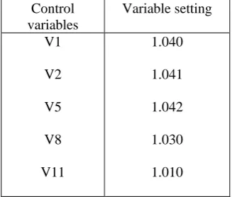
when compared to other given algorithms. The optimal values of the control variables along with the
minimum loss obtained are given in Table 1. Equivalent to this control variable setting, it was found
that there are no limit violations in any of the state variables.
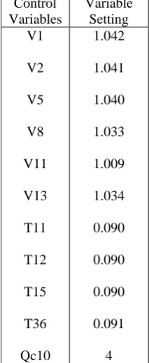
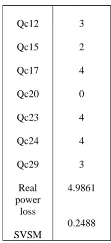
ORPD including voltage stability constraint problem was handled in this case as a multi-objective
optimization problem where both power loss and maximum voltage stability margin of the system were
optimized concurrently. Table 2 indicates the optimal values of these control variables. Also it is found
that there are no limit violations of the state variables. It indicates the voltage stability index has
increased to 0.2472 from 0.2488, an advance in the system voltage stability. To determine the voltage
security of the system, contingency analysis was conducted using the control variable setting obtained
in case 1 and case 2. The Eigen values equivalents to the four critical contingencies are given in Table
3. From this result it is observed that the Eigen value has been improved considerably for all
contingencies in the second case.
Table 1.Results of DEHS – ORPD optimal control variables
Control variables
Variable setting
V1
V2
V5
V8
V11
1.040
1.041
1.042
1.030
1.010
V13 T11 T12 T15 T36 Qc10 Qc12 Qc15 Qc17 Qc20 Qc23 Qc24 Qc29 Real power loss SVSM 1.040 1.03 1.03 1.0 1.0 3 2 2 0 3 4 4 3 4.4045 0.2472
Qc12
Qc15
Qc17
Qc20
Qc23
Qc24
Qc29
Real power
loss
SVSM
3
2
4
0
4
4
3
4.9861
0.2488
Table 3.Voltage Stability under Contingency State
Sl.No Contingency ORPD
Setting
VSCRPD
Setting
1 28-27 0.1410 0.1430
2 4-12 0.1658 0.1661
3 1-3 0.1774 0.1783
4 2-4 0.2032 0.2041
Table 4.Limit Violation Checking Of State Variables
State
variables
limits
ORPD VSCRPD
Lower upper
Q1 -20 152 1.3422 -1.3269
Q2 -20 61 8.9900 9.8232
Q5 -15 49.92 25.920 26.001
Q8 -10 63.52 38.8200 40.802
Q11 -15 42 2.9300 5.002
Q13 -15 48 8.1025 6.033
V3 0.95 1.05 1.0372 1.0392
V4 0.95 1.05 1.0307 1.0328
V6 0.95 1.05 1.0282 1.0298
V7 0.95 1.05 1.0101 1.0152
V9 0.95 1.05 1.0462 1.0412
V10 0.95 1.05 1.0482 1.0498
V12 0.95 1.05 1.0400 1.0466
V14 0.95 1.05 1.0474 1.0443
V15 0.95 1.05 1.0457 1.0413
V16 0.95 1.05 1.0426 1.0405
V17 0.95 1.05 1.0382 1.0396
V18 0.95 1.05 1.0392 1.0400
V19 0.95 1.05 1.0381 1.0394
V20 0.95 1.05 1.0112 1.0194
V21 0.95 1.05 1.0435 1.0243
V22 0.95 1.05 1.0448 1.0396
V23 0.95 1.05 1.0472 1.0372
V24 0.95 1.05 1.0484 1.0372
V25 0.95 1.05 1.0142 1.0192
V26 0.95 1.05 1.0494 1.0422
V27 0.95 1.05 1.0472 1.0452
V28 0.95 1.05 1.0243 1.0283
V29 0.95 1.05 1.0439 1.0419
V30 0.95 1.05 1.0418 1.0397
Table 5.Comparison of Real Power Loss
Method Minimum
loss
Evolutionary
programming[34]
5.0159
Genetic algorithm[35] 4.665
Real coded GA with
Lindex as
SVSM[36]
4.568
Real coded genetic
algorithm[37]
4.5015
Proposed DEHS
method 4.4045
8. Conclusion
In this paper a novel approach DEHS algorithm used to solve optimal reactive power dispatch
problem.The performance of the proposed algorithm has been demonstrated through its voltage
stability assessment by using modal analysis method and is effective at various instants following
system contingencies. Also this method has a good performance for voltage stability Enhancement of
large, complex power system networks. The effectiveness of the proposed method is demonstrated on
IEEE 30-bus system.
References
[1] O.Alsac,and B. Scott, “Optimal load flow with steady state security”,IEEE Transaction. PAS -1973,
pp. 745-751.
[2] Lee K Y ,Paru Y M , Oritz J L –A united approach to optimal real and reactive power dispatch ,
IEEE Transactions on power Apparatus and systems 1985: PAS-104 : 1147-1153
[3] A.Monticelli , M .V.F Pereira ,and S. Granville , “Security constrained optimal power flow with
post contingency corrective rescheduling” , IEEE Transactions on Power Systems :PWRS-2, No. 1,
pp.175-182.,1987.
[4] Deeb N ,Shahidehpur S.M ,Linear reactive power optimization in a large power network using the
decomposition approach. IEEE Transactions on power system 1990: 5(2) : 428-435
[5] E. Hobson ,’Network consrained reactive power control using linear programming, ‘ IEEE
Transactions on power systems PAS -99 (4) ,pp 868=877, 1980
[6] K.Y Lee ,Y.M Park , and J.L Oritz, “Fuel –cost optimization for both real and reactive power
dispatches” , IEE Proc; 131C,(3), pp.85-93.
[7] M.K. Mangoli, and K.Y. Lee, “Optimal real and reactive power control using linear programming”
, Electr.Power Syst.Res, Vol.26, pp.1-10,1993.
[8] S.R.Paranjothi ,and K.Anburaja, “Optimal power flow using refined genetic algorithm”,
Electr.Power Compon.Syst , Vol. 30, 1055-1063,2002.
[9] D. Devaraj, and B. Yeganarayana, “Genetic algorithm based optimal power flow for security
enhancement”, IEE proc-Generation.Transmission and. Distribution; 152, 6 November 2005.
[10] C.A. Canizares , A.C.Z.de Souza and V.H. Quintana , “ Comparison of performance indices for
detection of proximity to voltage collapse ,’’ vol. 11. no.3 , pp.1441-1450, Aug 1996 .
[11] J. H. Holland, Adaptation in Natural and Artificial Systems, MIT Press, 1975
[12] T. B¨ack, F. Hoffmeister, H. Schwefel, A survey of evolution strategies, In Proceedings of the
Fourth International Conference on Genetic Algorithms and their Applications, 1991, 2-9
[13] J. Koza, Genetic Programming: On the Programming of Computers by Means of Natural
Selection, MIT Press, Cambridge, MA, 1992
[14] L. Fog, Evolutionary Programming in Perspective: The Top-down View, IEEE Press, USA, 1994
[15] R. Storn, K. Price, Differential Evolution – A Simple and Efficient Adaptive Scheme for Global
Optimization over Continuous Spaces, Technical Report TR-95-012, International Computer Science
Institute, Berkeley, CA, 1995
[16] S. Kirkpatrick, C. Gelatt, M. Vecchi, Optimization by simulated annealing. Science 220 (4598),
1983, 671-680
[17] R. C. Eberhart, J. Kennedy, A new optimizer using particle swarm theory, in: Proceedings of the
Sixth International Symposium on Micromachine and Human Science, Nagoya, Japan, 1995, 39-43
[18] J. Kennedy, R. C. Eberhart, Particle swarm optimization. Piscataway: Proceedings of IEEE
International Conference on Neural Networks, IEEE Press, NJ 1995, 1942-1948
[19] C. M. Bishop, Neural Networks for Pattern Recognitionm, Oxford University Press, 1995
[20] D. Goldberg, Genetic Algorithms in Search, Optimization and machine learning, Addison-Wesley,
1989
[21] K. Price, R. Storn, J. Lampinen, Differential Evolution – A Practical Approach to Global
Optimization, Springer, Heidelberg, 2005
[22] R. Storn, System design by constraint adaptation and differential evolution. IEEE Transactions on
Evolutionary Computation 3(1), 1999, 22-34
[23] R. Storn, Digital Filter Design Program FIWIZ, http://www.icsi.berkeley.edu/ storn/fiwiz.html,
2000
[24] T. Krink, B. Filipic, G. B. Fogel, R. Thomsen, Noisy optimization problems – A particular
challenge for differential evolution. In: Proceedings of 2004 Congress on Evolutionary Computation,
IEEE Press, Piscataway, 2004, 332-339
[25] Z. Geem, J. Kim, G. Loganathan, A new heuristic optimization algorithm: Harmony search,
Simulation 76(2), 2001, 60-68
[26] Z. Geem, C. Tseng, Y. Park, Harmony search for generalized orienteering problem: Best touring
in China, Springer Lecture Notes Comput, Sci 3412, 2005, 741-750
[27] J. H. Kim, Z. Geem, E. S. Kim, Parameter estimation of the nonlinear muskingum model using
harmony search, J. Am. Water Resour. Assoc 37(5), 2001, 1131-1138
[28] Z. Geem, J. H. Kim, G. V. Loganathan, Harmony search optimization: Application to pipe
network design, Int. J. Model. Simulat 22(2), 2002, 125-133
[29] Z. Geem, Optimal cost design of water distribution networks using harmony search, Engrg. Optim
38(3), 2006, 259-280
[30] K. S. Lee, Z. Geem, A new structural optimization method based on the harmony search
algorithm, Comput, Struct 82(9-10), 2004, 781-798
[31] T. W. Liao, Two hybrid differential evolution algorithms for engineering design optimization,
Applied Soft Computing 10(4), 2010, 1188-1199
[32] M. Mahdavi, M. Fesanghary, E. Damangir, An improved harmony search algorithm for solving
optimization problems, Applied Mathematics and Computation 188, 2007, 1567-1579 1900
[33] X. Liu et al. , A hybrid Harmony search approach Based on Differential Evolution, Journal of
Information & Computational Science 8: 10 (2011) 1889-1900.
[34] Wu Q H, Ma J T. Power system optimal reactive power dispatch using evolutionary programming.
IEEE Transactions on power systems 1995; 10(3): 1243-1248 .
[35] S.Durairaj, D.Devaraj, P.S.Kannan ,’ Genetic algorithm applications to optimal reactive power
dispatch with voltage stability enhancement’ , IE(I) Journal-EL Vol 87,September 2006.
[36] D.Devaraj ,’ Improved genetic algorithm for multi – objective reactive power dispatch problem’
European Transactions on electrical power 2007 ; 17: 569-581.
[37] P. Aruna Jeyanthy and Dr. D. Devaraj “Optimal Reactive Power Dispatch for Voltage Stability
Enhancement Using Real Coded Genetic Algorithm” International Journal of Computer and Electrical
Engineering, Vol. 2, No. 4, August, 2010 1793-8163.
K. Lenin has received his B.E., Degree, electrical and electronics engineering in 1999 from university of madras, Chennai, India and M.E., Degree in power systems in 2000 from Annamalai University, TamilNadu, India. At present pursuing Ph.D., degree at JNTU, Hyderabad,India.
Bhumanapally. RavindhranathReddy, Born on 3rd September,1969. Got his B.Tech in Electrical & Electronics Engineering from the J.N.T.U. College of Engg., Anantapur in the year 1991. Completed his M.Tech in Energy Systems in IPGSR of J.N.T.University Hyderabad in the year 1997. Obtained his doctoral degree from JNTUA,Anantapur University in the field of Electrical Power Systems. Published 12 Research Papers and presently guiding 6 Ph.D. Scholars. He was specialized in Power Systems, High Voltage Engineering and Control Systems. His research interests include Simulation studies on Transients of different power system equipment.
M. Surya Kalavathi has received her B.Tech. Electrical and Electronics Engineering from SVU, Andhra Pradesh, India and M.Tech, power system operation and control from SVU, Andhra Pradesh, India. she received her Phd. Degree from JNTU, hyderabad and Post doc. From CMU – USA. Currently she is Professor and Head of the electrical and electronics engineering department in JNTU, Hyderabad, India and she has Published 16 Research Papers and presently guiding 5 Ph.D. Scholars. She has specialised in Power Systems, High Voltage Engineering and Control Systems. Her research interests include Simulation studies on Transients of different power system equipment. She has 18 years of experience. She has invited for various lectures in institutes.