A taxonomy of camera calibration and video
projection correction methods
Radhwan Ben Madhkour, Matei Mancas, Thierry Dutoit
1Numediart Institute, Engineering Faculty (FPMs), University of Mons, Belgium
Abstract
This paper provides a classification of calibration methods for cameras and projectors. From basic homography to complex geometric calibration methods, this paper aims at simplifying the choice of the methods to perform a calibration regarding the complexity of the setup.
The classical camera calibration methods are presented. A comparison gives the pros and cons for each method.
For the projector calibration, the homography, the structured light methods and the geometric calibration are presented. Every general approach for the projector calibration is studied and the limitations of each method are given. Each approach is described through the main reference method. A classification of each projector calibration approach is given.
Keywords: projector calibration
1. Introduction
Video projectors are initially designed to make simple projections on smooth flat walls or screen surfaces. However, a variety of applications need projections on more and more complex surfaces which may also be in movement. Thus projections on buildings (mappings), on tables and complex objects, on moving objects and even on people bring novel experiences and interfaces into our lives.
Those applications need complex projections on moving objects or complex surfaces and outdoor or indoor setups. In addition, for most of the applications a single video projector is not enough and several projectors must be used together to cover the whole projection area. Those new uses of video projectors imply different projector calibration techniques depending on the use case. In the last years, number of new calibration methods were published having different interesting features.
In this paper, we present a classification of the state of the art of the calibration techniques. The goal is to provide useful information for both specialists and simple users (like people from industry or artists who need those techniques for their applications like mappings on buildings or novel HCIs). For that
∗
Corresponding author. Email:5DGKZDQ%HQ0DGKNRXU#XPRQVDFEH
purpose, we focused on describing for each family of methods the main reference without listing all the references which propose slight modifications of those methods.
In section 2, we present an overview of camera and projector calibration. In section 3, we present classical camera calibration methods. In section 4, we present a classification of the state-of-the-art approaches which is very useful to chose a method depending on the needed installation setup (in terms of difficulty or how much automatic it is) and depending on the features needed (projection on a plane or a complex surface, on a moving object or a static surface). In section 5, we discuss the validation of those methods and we finally conclude in section 6.
2. Camera/Projector
model
The calibration process is an estimation of the parameters of a model representing the camera or the projector. In the case of camera or projector calibration, the standard model is the so-called "pinhole model". The pinhole model is described more in-depth in [1]. A video projector mathematically differs from a camera only in the light ray direction[2], so the pinhole model can describe (at a sign difference) both cameras or video projectors. It is mathematically described by equation 1.
1
Received on 11 June 2014, accepted on 29 January 2015, published on 27 February 2015
Copyright © 2015 Radhwan Ben Madhkour et al., licensed to ICST. This is an open access article distributed under the terms of the Creative Commons Attribution licence (http://creativecommons.org/licenses/by/3.0/), which permits unlimited use, distribution and reproduction in any medium so long as the original work is properly cited.
doi: 10.4108/ct.2.2e2
world
position where the pixel x lights up. The matrix K is called the projector calibration matrix. It is defined by:
K=
fu 0 u0 0 fv v0
0 0 1
(2)
where fu,fv are the focal lengths in the u and v
directions respectively and (u0, v0), the principal point coordinates. The focal length is the distance between between the image plane and the camera center. The principal point is the intersection between the optical axis (zaxis) and the image plane. [R|t] is the "pose" of the projector and represents the transformation (change of coordinates frame) from the world to projector coordinates. This transformation is composed of a rotationR and a translationt. The pinhole model can be extended to take into account the lens distortions.
3. Classical camera calibration methods
In this section, we will discuss the standard camera calibration methods: DLT [1], Tsai [3], Heikkila [4] and Zhang [5].
3.1. Direct Linear Transform (DLT)
Idea. The Direct Linear Transform is the straight for-ward solution to the calibration problem. The algorithm builds an equation system from the fundamental equa-tions of the pinhole model (eq. 1). The system of the formAx= 0 is solved with a least squares method.
More details. A cross product of each term of equation 1gives:
xi ×P Xi =
yiP3TXi−wiP2TXi
wiP1 T
Xi−xiP3 T
Xi
xiP2TXi −yiP1TXi
=xi ×xi = 0 (3)
0T −wiXT
i yiXiT
wiXiT 0T −xiXiT
−yiXT
i xiXiT 0T
P1 P2 P3
= 0 (4)
In this equation, X is a 3D coordinate in the world coordinate frame and x (x, y, w) is the coordinate of its projection on the image plane. PiT is the ith
line of P and 0T is the null vector. P has twelve parameters but only eleven are independent. Indeed, the matrixP is homogeneous and only the ratio between each value is important [1]. A set of correspondences between 3D coordinates and their 2D projection gives (BLUB) a system of equations that is solved with the singular value decomposition (SVD). To retrieve the correspondences, a 3D pattern is used.
P =
fxr1+u0r3 fxtx+u0tz
fyr2+v0r3 fyty+v0tz
r3 tz
r3 = p3 u0 = pt1p3
fx =
q
pT1p1−u02 tx = (p14−u0tz)/fx
r1 = (p1−u0r3)/fx
tz = p34
v0 = pt1p3
fy =
q
pT2p2−v02 ty = (p24−v0tz)/fy
r2 = (p2−v0r3)/fy
(5) The second approach is based on the QR decomposi-tion of P [1]. QR decomposidecomposi-tion breaks a matrix into a upper triangular matrix Q and a rotation matrix R. We have
P =K[R|t] = [KR|Kt] = [M|Kt]
where M is the product of K, an upper triangular matrix, and R, a rotation matrix. If we apply QR decomposition on M, we retrieve K and R. The translation vector is found from the last column ofP.
t=K−1P4
Procedure. The calibration needs the combination of pixel and 3D coordinates to be performed. Most of the time, a 3D pattern, like a cube shown on figure1, is used to acquire the set of correspondences. While a single capture give the calibration, more correspondences from other points of view lead to a better accuracy.
3.2. Tsai and Heikila: two evolutions of the DLT
algorithm
The algorithm proposed by Tsai [3] is based on a modification of the basic equations of the pinhole model. Tsai introduces a term to model the distortion. In order to maintain the linearity of the equations, only the radial part of the distortion is modelled. A Levenberg-Marquard non linear optimization is used only for f,tz,k1etk2.
Imposing the principal point as known simplifies the calibration problem. We will discuss the impact of this hypothesis on the projector geometrical calibration in section4.3.
This method offers a solution to the calibration based on a set of coplanar points or non coplanar 3D points. Both algorithms are slightly different and the next section will focus on the general method.
The algorithm is decomposed in two steps. The first estimates the matrix R,tx,tyandsx. The second retrieve
f, tz. Finally, a non linear optimization is applied to
Figure 1. Non planar pattern used to calibrate a camera with Heikkila’s method (image credits [4])
Heikkila has improved the DLT by introducing a global optimization and the estimation of the distortion coefficients. It is decomposed into four steps:
DLT the linear solution to calibration problem pre-sented in section3.1.
Non linear optimization A Levenberg Marquardt least-squares optimization method is applied to reduce the reprojection error, the error between the measured 2D points and the reprojected 3D points using the estimated model.
Solution refinement The parameters are refined to align the circle center of the pattern used to retrieve 2D|3Dcorrespondences.
Distortion the radial and tangential components of the lens distortions are estimated.
The calibration method needs a non planar pattern to perform (fig.1). One view of the pattern is sufficient to calibrate but the addition of views increases the results accuracy.
3.3. Zhang’s method
Zhang’s algorithm is currently the most popular for the camera calibration. The method uses a plane to achieve the camera calibration. The standard pattern used is a chess board. Indeed, the size of each square of the chess board is easily measured and the the pattern itself is easily automatically detected. Moreover, the method gives good results and the calibration process is simple. Zhang’s algorithm can be seen as a particular case of the planar autocalibration problem [6, 7]. Triggs [6] showed that without assuming the 3D coordinates known, the inter-image homographies are sufficient to perform the calibration.
Idea. A homography can be calculated between the image plane and the pattern. This homography imposes two constraints. To perform the intrinsic calibration, six parameters have to be estimated. Nevertheless, the matrix is homogeneous and only five parameters are independent and need to be calculated. Hence, the minimum number of pattern images is three. If the skewness is set to zero (square pixel hypothesis), this
(a) (b)
Figure 2. Pattern corners detection
number is reduced to two. Nevertheless, in practice, a good calibration is generally achieved with more than five different views.
The intrinsic and extrinsic parameters are estimated first. Then, the distortion coefficient are calculated. Finally, all parameters are refined using a non linear optimization.
Procedure. Zhang’s algorithm requires images of a planar pattern form different point of view. Figure 2 shows two examples of the planar pattern capture and its corners detection.
In practice, two images are sufficient to achieve the calibration. Nevertheless, at least four views are required to get a good accuracy.
3.4. Tools
Implementations of these methods are available. In C++, the OpenCV library gives an implementation of Zhang algorithm. In Matlab, Bouguet’s calibration toolbox [8] provides a set of functions for camera calibration and an easy-to-use calibration tool. Heikkila provides a Matlab toolbox that can be integrated with the Bouguet’s tool. Tsai’s implementations by [9] is no more available. [10] proposes a Matlab implementation but without the final non linear optimization.
3.5. Comparaison
Table1presents a comparison of the camera calibration methods presented in previous sections. The robustness represents how the methods behave with errors. Accuracy is the overall accuracy of the method. The simplicity of the intrinsic parameters and the pose estimation is also evaluated. The simplicity measure is based on the comparison of the procedures.
Robustness and accuracy of the methods have been studied by [11]. They concluded that Zhang is more robust to noise than other methods. Accuracy is difficult to estimate on real data because of the lack of a precise ground truth. While in theory, Tsai and Heikkila are supposed to perform better than Zhang, Zhang gives better results in practice, where measured points are subject to noise.
3 EAI Endorsed Transactions on Creative Technologies
Table 1. Comparison of Heikkila, Tsai and Zhang methods in terms of robustness, accuracy and how easy the intrinsic and pose calibration is performed
Indeed, Zhang imposes a planar constraint to the measured points while Tsai and Heikkila process them separately. In terms of use, Zhang estimates the pose for every view of the calibration board. Hence, unless one of the calibration board positions corresponds to the world coordinate frame needed, the extrinsic calibration have to be performed with the camera at the right place after the intrinsic calibration is done. Pose and intrinsic calibration with Tsai and Heikkila’s methods can be done together but a 3D calibration pattern or a 3D measurement tool is needed to perform the calibration. Generally, Zhang’s method is the one chosen to calibrate intrinsic parameters of a camera. Pose calibration algorithms like PnP [12] are then used to estimate a specific world to camera transform.
4. Projector calibration methods
A projector can be seen as a camera that projects light instead of acquiring it. From a mathematical point of view, the same relation and model can be applied on it. Nevertheless, to correct a projection, the type of surface and the presence of movement influence the choice of the method. A full calibration like for the cameras is not always needed. The goal of this section is to give an overview of the methods available to correct a projection from the linear relation to the complete scene modeling. A practical guide gives some hints to simplify the choice of the method according to the setup needed in practice.
4.1. Homography: a linear correction
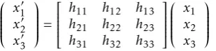
An homography (eq. ??) is a relation that maps coordinates from two planes. In the projection, it is used to warp the image to rectify its position and orientation to fit to some constraints like complex shapes.
x01 x02 x03
=
h11 h12 h13 h21 h22 h23 h31 h32 h33
x1 x2 x3
(6)
As the relation is linear, the image deformation is correct only on a given plane. The mapping of complex images on complex surfaces is difficult to achieve without heavy manual fine-tuning.
Figure3 shows the effect of an homography (linear mapping) on an image.
(a) (b)
Figure 3. Homography results. (a) Original image. (b) Deformed image
4.2. Structured light: a pixel by pixel correction
The structured light method needs a camera to generalize the mapping to complex surfaces. Structured light retrieves the correspondences between the pixel of the projector and the camera. It is calculated pixel by pixel and the result is an (u,v) map that identifies the position of the projector pixel on the camera view, regardless the shape of the surface. In this case, the correction will always be perfect in the camera point of view.The method encodes the position of each projector pixel in a set of images (called patterns). The number of images depends on the coding method and the projector resolution. The patterns are projected and an image of each projected pattern is acquired by the camera. To calculate the (u,v) map, the images are decoded.
Multiple methods of coding exists. [13] and [14] present a review of structured light methods. In the next section, we will describe briefly two classical methods, the Gray code and the three phase shift. We will also present other approaches that give better results.
Gray coded patterns. Each pixel is coded in a unique binary code that has only one bit different with each neighbor. Every bit of this code is used to create a binary image. The encoding gives a set of horizontal (vertical) patterns that encodes the vertical (horizontal) position of the pixel. An example of patterns created using the Gray code is shown on fig.4.
Three phase shift. The pixel coordinate influences the phase of a sinusoidal function [15]. Instead of a binary set of images, the patterns obtained are in gray level (fig. 5).
Figure 4. A set of Gray coded patterns
Figure 5. A set of three phase shift patterns
give sub pixel precision. For this reasons, Gray coded and three phase shift methods are combined [16]. Recently, Couture et al. [17] proposed a new approach to unstructured light. Unstructured light pattern does not encode directly the position of the projector pixels. The correspondences are obtained through a matching method like in stereoscopy. The proposed pattern has particular properties that gives better results.
4.3. Geometric calibration: a correction through the
scene model
Homography is widely used in the case of a planar surface. To project on complex surfaces, structured light is used to map pixel by pixel the image on the surface. When the complex surfaces are moving, both methods fail to correct the projection without re-calibrating the system. In this case, the solution is to model the scene. The projection is the result of the real-time rendering of a model of the scene. The projector is modeled by a virtual camera that observes the model of the projection surface from the projector point of view. Geometric calibration gives the parameters of the projector model. The scene model can be acquired in real-time with a depth camera. If a 3D model of the scene is available, the model has to be adapted in real-time using tracking techniques.
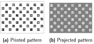
Zhang-based method. Audet and Okotumi’s algorithm [18] is based on Zhang calibration method. It uses a planar pattern to calibrate the projector. Nevertheless, instead of a standard chess board, the black and white square are replaced by BCH markers of ArToolKit [19]. In addition, only half of the markers are printed on the plane. The rest of the pattern is projected.
The proposed algorithm is based on Zhang’s method. Hence, the projected pattern has to be aligned with the printed one so that the position of the projector pixels
(a)Printed pattern (b)Projected pattern
Figure 6. Both parts of the pattern (image credits[18])
(here the markers corners) and their 3D coordinates can be calculated.
An homography Hpanc is calculated between the
camera and the calibration pattern. This homography is estimated thanks to the printed markers. Eq.7shows the relation between a point xpan on the calibration board
andxc, the corresponding point on the image plane.
xpan=Hpancxc (7)
Hpancis the same homography as in eq.??for Zhang’s
calibration. In the same way, an homography connects the pixels of the projector yp and the points on the
calibration boardypan(eq.8).
ypan =HpancHcpyp (8)
As we have no a priori knowledge on the projected pixels position on the calibration board, the projection has to be aligned with the printed pattern on the board. An homographyHpcorrects the points position (eq.9).
ypan0 =HpancHcpy
0
pavec y
0
p=Hpyp (9)
Figure7gives the calibration procedure.
• Project a part of the pattern
• Align the projected pattern with the one on the calibration board using an homograhy
• Refine the estimated homography
• If the error is smaller than a threshold, the points can be used as entries to the Zhang’s calibration algorithm.
General planar autocalibration. Drareni et al. [20] pro-posed a calibration method based on the camera planar autocalibration described by Triggs [6]. Triggs showed in that even if the structure of the scene is not known as in the Zhang’s case, the inter-image homo-graphies are sufficient to achieve the calibration. The inter-projector homographies are derived from the the camera-projector homographies (eq.10).
Hpi→pj = Hw→pjH −1
w→pi
= Hc→pjHw→c(Hc→pjHw→c)−1 = Hc→pjHc−→1pi
(10)
5 EAI Endorsed Transactions on
Figure 7. Diagram of the calibration procedure (image credits
[18])
In this equation, Hc→w is the homography used to calibrate a camera with Zhang’s approach but since there is no chessboard or pattern, this homography is unknown. As usual, a numerical optimization is used to solve the calibration problem. The optimization is initialized in the same way as Zhang or Triggs, ie. solving a system of equations built from two constraints using the image of the absolute conic.
In practice, the algorithm requires multiples images of a projected chess pattern from different projector positions.
Epipolar geometry based method. The approach proposed by Yamazaki et al. [21] is based on the epipolar geometry. The algorithm combines accurate projector to camera correspondences acquired with structured light and the epipolar geometry to achieve the calibration. As Tsai’s camera calibration algorithm, the method supposes the principal point as known. The projector model is slightly simplified by settingfx=fy=f.
Epipolar geometry gives an equation, the epipolar constraint, that links two vision devices.
(u1, v1,1)F(u2, v2,1)T = 0 (11)
In this equation, (un, vn,1) are the pixel coordinate
of a 3D point observed by the nth device. F is 3x3 matrix called the fundamental matrix. If the radial and tangential distortions are introduced, eq.11becomes:
(u12+v12, u1, v1,1)R(u22+v22, u2, v2,1)T = 0 (12)
In this equation, R is a 4x4 matrix called the radial fundamental matrix. The R matrix is determined with 15 correspondences. If the center of distortion is supposed known (equal to the principal point), R can be decomposed to retrieveF. Eq.13[22] gives the focal lengths fromFand the principal pointspcandpp.
Figure 8. Diagram of the calibration procedure (image credits
[23])
fp2=− pT
c[ec]xIˆ3FTpppTcFpc
pTc[ec]xIˆ3FTIˆ3Fpc fc2=−
pTp[ep]xIˆ3FTpcpTpFpp
pT
p[ep]xIˆ3FTIˆ3Fpp
(13)
As F andK are known, the essential matrixE gives the extrinsic parameters.
E = [t]xR
= Kp
−T FKc
−1 (14)
In practice, this direct solution is not used because eq.13is sensitive to errors. The solution is found using a non linear optimization method. The initial guess is estimated as follows:
• Set initial value to the principal points and focal lengths. The focal lengths are set to the diagonal length of projector and camera images.
• Estimate R by running RANSAC on the structured light correspondences.
• Decompose R to F and E. The correction of E (set two singular values to 1 and the last to 0 [1]) gives a better guess of F.
The calibration is performed automatically but up to a global scale.
DLT-based calibration method. Ben Madhkour et al. [23] proposed a method combining a RGBD camera and structured light accurate correspondences. Figure 8 gives the process of the calibration.
4.4. Comparaison
Table 2 shows the comparison of Audet et al. [18], Yamazaki et al. [21], Ben Madhkour et al. [23] and Draréni et al.[20]. The categories are the same as in table 1.
Audet and Draréni methods perform better than the other methods. By imposing a planar constraint, this methods are more robust and accurate. In practice, in the case of Draréni, the use of a general planar surface without any printed pattern simplifies the calibration process. Nevertheless, Yamazaki [21] and Ben Madhkour [23] automatize the process of calibration. [21] automation is achieved with the model simplification and the principal point a priori knowledge. [21] does the calibration up to a global scale and the size of an object or the distance of a point is needed to determine the scale factor. Ben Madhkour et al. [23] fully automatize the process by using a RGBD camera instead of a 2D camera. The pose is determined at the same time as the intrinsic parameters. In terms of simplicity of use, Ben Madhkour et al. [23] doesn’t need any human intervention or a priori knowledge.
This section aims at giving some hints on how to choose the right method to perform a complex projection given user’s constraints (projection surface type, easy-to-use, accurate, ...).
Projection surface type. The type of surface influences the choice of the method to correct a projection. A projection on a set of planar surfaces can be performed well enough with a simple homography correction. More complex surfaces require more powerful methods. The choice of the method to be used depends on the fact that the surface is static or dynamic (the object where the projection is done moves).
Dynamic or static surface. The projection on a static complex surface can be achieved using structured light. There are several methods of structured light to achieve pixel to pixel mapping. One of the best is Couture et al. [17]. If the surface is moving, the geometric calibration of the projector is needed. Planar calibration gives the best accuracy. The geometric calibration will correct the projection via a 3D rendering of the modeled surface. Since a 3D model and projector model are required, the use of a RGBD camera gives the 3D model and highly simplifies the procedure like in Ben Madhkour et al. [23].
Easy to use. The choice of the method must be
determined by the complexity of the setup. Indeed, while structured light or geometric calibration allows the projection on planar surfaces, the use of the homography is way simpler in this case. The tools are simple and no camera is required. In the case of complex surfaces, we propose to avoid "Gray coded patterns" because of its poor robustness against
reflections. Combinations of "Gray coded patterns"’ and "three phase shift" [16] achieve better results. If the surface is moving, Ben Madhkour et al. [23] method simplifies the calibration process by combining the structured light and the RGBD camera.
Accuracy. Accuracy can be influenced by multiple parameters:
• algorithm
• quality of the tools
• user
The homography is an accurate method in the case of linear correction. Errors can be introduced by the user that selects wrong destination points.
The structured light accuracy is influenced by the choice of the pattern and the complexity of the projection surface. Recent work from Couture et al. [17] proposed a versatile method that is less influenced by reflection than other methods.
The geometric projector calibration accuracy is mostly influenced by the algorithm and the tools. Audet et al. [18] and Draréni[20] are the most accurate method in the case of intrinsic calibration.
5. Projector calibration methods validation
Structured light and geometric calibration are objec-tively compared with the ground truth using the root mean square error (RMSE) or the reprojection RMSE.
For structured light method, the validation is based on a known surface. In [14], a planar surface is used. The 3D reconstruction obtained with the calibrated couple of projector and camera is compared with the plane. In the case of Martin [24], the reference is acquired with a 3D laser scanner.
When comparing geometric calibration, the methods evaluation is performed with the data used to calibrate. The RMSE is used to compare data from reprojected with the estimated model and the original data. Audet et al. gives a table RMSE for different methods [18]. Draréni et al. [20] obtained error values similar to Audet. Yamzaki [21] does not provide values of RMSE but uses [18] as ground truth. Ben Madhkour et al. reached a higher RMSE value that is explained by the use of Gray coded structured light, the precision from a RGBD camera (like the Microsoft Kinect sensor) and the DLT.
6. Conclusion
In this paper, we have described classical methods for camera calibration and video projector correction. Four algorithms have been presented: the direct linear algorithm, the Heikkila [4] and Tsai [3] modifications and Zhang [5]. These methods have been compared and
7 EAI Endorsed Transactions on
Drareni [20] *** *** *** *
Table 2. Comparison of projector calibration methods in terms of robustness, accuracy, simplicity of intrinsic and pose calibration
a classification regarding their robustness, accuracy and the simplicity of intrinsic and pose calibration has been proposed.
For the projector, popular methods for video projection correction have been described. Three approaches have been presented: the homography, the structured light and the geometric calibration. In the case of the structured light, we described the Gray code and the three phase shift and presented more advanced methods. For the geometric calibration, four methods to achieve the modeling of the projector have been described. Finally, a comparison of the methods through their performance and the practical point of view has been given. We gave an overview of the methods and the best methods to choose regarding the type of projection surface, the presence of movement in the scene and how easy to use the method is.
Finally we described two validation measures for structured light and geometric method and discussed the geometric methods validation.
The number of potential applications of adaptative projection is growing and more and more HCI will use those techniques in indoor conditions (homes, museums, ...). The future of these applications is a method which is simple (easy to install and with automatic setup) and which works for complex and moving surfaces. While the accuracy of the method is important, subjective measures are the key of a well accepted application which does not sacrifice simplicity to gain in accuracy which is not even perceived by the users. The main challenge for future projector calibration methods is to find the optimal balance between perceived accuracy for a given application and setup simplicity.
References
[1] Hartley R, Zisserman A. Multiple view geometry in computer vision. Cambridge University Press; 2004. [2] Kimura M, Mochimaru M, Kanade T. Projector
calibration using arbitrary planes and calibrated camera. In: Proceedings of the 2007 IEEE Computer Society Conference on Computer Vision and Pattern Recognition (CVPR’07). IEEE Computer Society; 2007. p. 1–2. [3] Tsai RY. An efficient and accurate camera calibration
technique for 3D machine vision. In: Computer Vision and Pattern Recognition; 1986. .
[4] Heikkila J. Geometric camera calibration using circular control points. IEEE Transactions on Pattern Analysis and Machine Intelligence. 2000;22(10):1066–1077. [5] Zhang Z. A flexible new technique for camera
calibration. IEEE Transactions on Pattern Analysis and Machine Intelligence. 2000;22(11):1330–1334.
[6] Triggs B. Autocalibration from Planar Scenes. In: 5th European Conference on Computer Vision (ECCV 1998); 1998. p. 89–105.
[7] Sturm P, Maybank SJ. On Plane-Based Camera Calibra-tion: A General Algorithm, Singularities, Applications. In: IEEE Conference on Computer Vision and Pattern Recognition, CVPR’99, June, 1999. vol. 1. Fort Collins, CO, Etats-Unis: IEEE; 1999. p. 432–437.
[8] Bouguet JY. Camera Calibration Toolbox for Matlab; 2010. Available from: http://www.vision.caltech. edu/bouguetj/calib_doc/.
[9] Wilson R. Tsai calibration;. Available from:
http://www-cgi.cs.cmu.edu/afs/cs.cmu.edu/user/ rgw/www/TsaiCode.html.
[10] Daesik K. 3D computer vision: MATLAB Functions; 2012. Available from: http://www.daesik80.com/ matlabfns/matlabfns.htm.
[11] Sun W, Cooperstock R. An empirical evaluation of factors influencing camera calibration accuracy using three publicly available techniques. Mach Vision Appl. 2006 Mar;17(1):51–67.
[12] Lepetit V, Moreno-Noguer F, Fua P. EPnP: An Accurate O(n) Solution to the PnP Problem. International Journal of Computer Vision (IJCV). 2009;.
[13] Salvi J, Pagès J, Batlle J. Pattern Codification Strategies in Structured Light Systems. PATTERN RECOGNITION. 2004;37(4):827–849.
[14] Salvi J, Fernandez S, Pribanic T, Lladó X. A state of the art in structured light patterns for surface profilometry. Pattern Recognition. 2010;43(8):2666–2680.
[15] Huang PS, Zhang S. Fast three-step phase-shifting algorithm. Applied Optics. 2006 Jul;45(21):5086–5091. [16] Sansoni G, Carocci M, Rodella R. Three-Dimensional
Vision Based on a Combination of Gray-Code and Phase-Shift Light Projection: Analysis and Compensation of the Systematic Errors. Appl Opt. 1999 Nov;38(31):6565– 6573.
[17] Couture V, Martin N, Roy S. Unstructured Light Scanning to Overcome Interreflections. In: Proceedings of the 2011 International Conference on Computer Vision. ICCV ’11. Washington, DC, USA: IEEE Computer Society; 2011. p. 1895–1902.
2009;0:47–54.
[19] Wagner D, Schmalstieg D. ARToolKitPlus for Pose Track-ing on Mobile Devices. Institute for Computer Graphics and Vision, Graz University of Technology; 2007. Avail-able from: http://www.icg.tu-graz.ac.at/Members/ daniel/ARToolKitPlusMobilePoseTracking.
[20] Draréni J, Roy S, Sturm PF. Methods for geometrical video projector calibration. Machine Vision and Applications. 2012;23(1):79–89.
[21] Yamazaki S, Mochimaru M, Kanade T. Simultaneous Self-Calibration of a Projector and a Camera Using Structured Light. In: Proceedings of the 2011 IEEE Computer Society Conference on Computer Vision and Pattern Recognition (CVPR’11) - Workshops (Procams
2011). IEEE Computer Society; 2011. p. 67–74.
[22] Bougnoux S. From Projective to Euclidean Space Under any Practical Situation, a Criticism of Self-Calibration. In: Proceedings of the 1998 International Conference on Computer Vision. ICCV ’98; 1998. p. 790–798.
[23] Ben Madhkour R, Mancas M, Gosselin B. Automatic Geometric Projector Calibration - Application to a 3D Real-time Visual Feedback. In: Battiato S, Braz J, editors. VISAPP (2). SciTePress; 2013. p. 420–424.
[24] Martin N, Couture V, Roy S. Subpixel Scanning Invariant to Indirect Lighting Using Quadratic Code Length. In: The IEEE International Conference on Computer Vision (ICCV); 2013. .
9 EAI Endorsed Transactions on
![Figure 1. Non planar pattern used to calibrate a camera withHeikkila’s method (image credits [4])](https://thumb-us.123doks.com/thumbv2/123dok_us/8414313.1691859/3.595.323.528.90.189/figure-planar-pattern-calibrate-camera-withheikkila-method-credits.webp)
![Figure 8. Diagram of the calibration procedure (image credits[23])](https://thumb-us.123doks.com/thumbv2/123dok_us/8414313.1691859/6.595.331.531.94.203/figure-diagram-calibration-procedure-image-credits.webp)

