Linking Data According to Their Degree of Representativeness (DoR)

(1)

Research

Article

Linking Data According to Their Degree of

Representativeness (DoR)

Frédéric Blanchard

1,∗

, Amine Aït-Younes

1

, Michel Herbin

1

1_{Université de Reims Champagne-Ardenne, CReSTIC, UFR Sciences Exactes et Naturelles, Moulin de la Housse,}

BP 1039, 51687 Reims CEDEX 2, FRANCE

Abstract

Thiscontributionaddressestheproblemof extractingsomerepresentativedatafromcomplex datasetsand connectingthem in a directed graph.First wedefine a degree of representativeness(DoR) inspiredof the Bordavotingprocedure.Secondlywepresentamethodtoconnectpairwisedatausingneighborhoodsandthe DoRasanobjectivefunction.Wethenpresentcasestudiesasillustrativepurposes:unsupervisedgroupingof binaryimages,analysisofco-authorshipsinaresearchteamandstructurationofamedicalpatient-oriented database

Keywords: Miningcomplexdata,Representativeness,Graphbaseddataanalysis

Received on 31 August 2014; accepted on 30 November 2014; published on 04 June 2015

Copyright© 2015 FrédéricBlanchardetal.,licensedtoICST.Thisisanopenaccessarticledistributedunderthetermsof theCreativeCommonsAttributionlicense(http://creativecommons.org/licenses/by/3.0/),whichpermitsunlimited use,distributionandreproductioninanymediumsolongastheoriginalworkisproperlycited.

doi:10.4108/inis.2.4.e2

1. Introduction

The selection of a small subset from a dataset is a classical way for both reducing the cost of data

processing and improving the efficiency of data

analysis. In statistics, the process is called sampling. The selection of representative samples is generally based on a randomization process. Unfortunately this approach assumes implicitly or explicitly that data distributions are known. Then the statistical analysis often fails when exploring dataset with unknown distributions. In data mining, the goal is very different. The samples should define interesting patterns and structures to analyse the data set. Then each sample is

selected taking into account its ownrepresentativeness.

These samples are calledexemplars[1]. The extraction

of these representative elements presents a significant

interest in designing recommendation systems [2],

selecting leaders or specimens [3] for community

detection [4] or for customer Relationship analysis [5]. In this context, this paper proposes a new approach for extracting exemplars (i.e. representative elements) from a dataset and for linking data to visualize the

∗

Correspondingauthor.Email:[email protected]

structure of the dataset as a forest.

In the framework of data mining, the classical ways to determine representative elements refer to the task

of clustering [6]. The representative elements are

prototypes selected from a partition of the dataset into clusters. This approach assumes that the number of exemplars is equal to the number of clusters. Unfortunately when exploring a dataset, the number of clusters is unkown. If a cluster contains more than one sub-population, then only one prototype is extracted. But more than one exemplar is expected. Moreover the exemplars are real data extracted from the dataset. But the prototypes are often virtual elements that does not make sense. For instance the

classical k−_{means algorithm (see [}₇_{] for a review of}

clustering methods including k−_{means algorithm)}

(2)

from a dataset.

Most of the methods for extracting exemplars are iterative. That is the case when using the k-medoids

algorithm [7] for determining k exemplars. First k

exemplars are randomly selected from the dataset. Then the algorithm iteratively refines this set of exemplars. The afinity propagation method of Frey

and Dueck [1] also proposes to extract exemplars by

iterative process. Unfortunately the final elements proposed as exemplars are quite sensitive to the initial selection, they depend on input parameters and on the way to stop the iterative process. To circumvent this drawback, this paper proposes a one pass method to extract exemplars from a dataset without any assumption on the shape or the density of data

distribution (unlike in [8]). The method we propose

is only based on a relation that permits a pairwise comparison of data. Using this relation we define a

degree of representativeness (DoR). The exemplars are finally chosen as local maxima of the DoR. Then we show how to build a directed graph to visualize the organization of dataset around the exemplars as trees.

By fitting the locality parameter calledscale factor we

determine the exemplars at each scale that the user needs.

The new method we propose is deterministic. Thus each dataset leads to one specific set of exemplars. Some properties can indicate the ability of the method to reveal intrinsic structures of the dataset. Thus the paper study the stability and the robustness of our method to indicate this ability. When data is corrupted with noise or outliers, the selection of exemplars should be robust against such corruptions. When resampling the dataset, the stability of exemplars (i.e. the exemplars do not change when resampling) is another indication of the ability of the method to reveal dataset structures. Moreover our deterministic method gives one result at each scale. When the scale increase, we also study the variation of the set of exemplars and the forest we build on the dataset.

To sum up this paper proposes a new method for exemplar selection and it studies some of properties of the method. It is organized as follows. In the first section we introduce the context and expose our

method. We present the formal definition of degree of

representativeness(DoR) used to extract exemplars. The

notion ofstandardis defined when only one exemplar is

selected from the dataset. Then we show how to build a directed graph (more precisely a forest) to visualize the inherent structure of the dataset. For each definition we present some interesting and remarkable properties (robustness and stability).

The next section presents three case studies in very

different contexts. Firstly we apply our method on a

set of binary images. We compute scores and exemplars and build the forest that emphases the structure of the set. The second application concerns the analysis of authorship in a research laboratory. We exhibit a co-authoring network (the forest of the co-authors) that permits to visualize how researchers are really clustered and how they work together.

Last section is a brief conclusion that outlines our main contributions and that expose our current and future works.

2. Method

Let Ω be a set of n elements in a multidimensional

space. Let us describe the way we use to extract the

exemplars from Ω for structuring this set as a forest.

In this paper, the nelements are called objects. They

consist of qualitative, quantitative or mixed data. We

assume that Ωis only a relational dataset. We do not

need for any assumption on underlying distribution of data. We only use the relation for comparisons between objects.

2.1. Pairwise Valued Relation

Let us specify the relation. LetRbe a pairwise valued

relation onΩ.Ris defined by :

R: Ω×Ω → _R+

(x, y) 7→ _R₍_{x, y}₎

The use of such a pairwise valued relation is very classical in data processing. For instance, the distance is a special case of this kind of relation. But a distance is frequently not available when processing qualitative data. Thus a relation is more widespread than a distance for pairwise comparisons of objects. In this paper, the valueR(x, y) is also called thecostfromxtoy, indicating the generality of the relation.

The relation must follow three trivial properties.

• The relation must betotal. This means that each

pair of objects ofΩis valued byR.

• The relation must bepositive. The cost is a positive value for all pairs.

• The cost from x to x is null forall x (i.e. ∀_x∈

Ω, R(x, x) = 0)

Unlike a distance, the relation does not necessarily

respect the property of symmetry. R(x, y) may be

different from R(y, x). For instance, if the cost from a

point x to a point y is the time to go from x to y,

then the cost from y to x could differ from the first

(3)

dissimilarity index gives a classical example of such a relation which does not respect the triangle inequality.

x is dissimilar fromy with R(x, y) andy is dissimilar fromzwithR(y, z) butxcould be dissimilar fromzwith

R(x, z)> R(x, y) +R(y, z).

Such a relation can lead to a vote to designate exemplars within the dataset. Specifically, we can rank the objets

of Ω taking into account the relation to set up

votes between the objects themselves. The following subsection describes this procedure.

2.2. Degree of representativeness (DoR)

In this paper, we select an exemplar object from Ω

according to the Borda voting method [9]. But firstly, we transform values of the relation into ranks [10][11][12].

Let us define these ranks. Letxbe an object ofΩ. All

objects can be sorted by the ascending order of their costs relative to x. Let us note Rkx(y) the rank of y

relative tox. Then the ranks are obtained when sorting

the set{_R₍_{x, z}₎_/z∈Ω}_{. Using Borda method [}₉_][₁₃_{], the}

objectxassigns a relative score to all objects ofΩ. The scoreScxrelative toxis defined by:

∀_y∈_Ω_{, Sc}_x₍_y_{) =}_n−_Rk_x₍_y₎

where n is the number of objects in Ω. Thereby the

relative score is an integer and it lies between 0 and

n−_{1. The lower the cost from} _x _to _y_{, the higher the}

score ofyrelative tox.

Computing all relative scores, each objectxreceivesn

scores corresponding to the votes of all objects ofΩ(i.e. thenvaluesScy(x) withy∈Ω). Then the relative scores

are aggregated to define thedegree of representativeness

(DoR) of data. The DoR is finally used as an objective function to choose the winner of the voting procedure. The aggregate score is defined by:

DoR : Ω → _R+

x 7→ _Aggreg

y∈_Ω(Scy(x))

In this paper, the aggregation function is the mean

function.

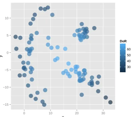
Let us observe the DoR in a simulated dataset.

Figure1displays an example of a dataset with 120 two

dimensional random samples (A). Euclidean distance is used as the pairwise valued relation between samples. The respective DoR (B) confirm that the score increases when the sample approaches the center of the dataset, i.e. in the midst of this one.

2.3. Standard

The object with highest DoR is called standard. The

standard is usefull when only one exemplar is expected

for resuming the datasetΩ.

−15 −10 −5 0 5 10

0 10 20 30

x

y

30 40 50 60

DoR

Figure 1. Example of a dataset with 120 random samples (A)

and their respective DoR (B). The DoR increases in the midst of the dataset

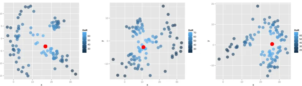
Let us give three examples of standard. The figure 2

shows the graphical representations of three datasets A, B, and C. Each dataset is randomly generated and

contains 100 data (n= 100) and two features x and

y. The DoR is computed using Euclidean distance as

pairwise valued relation. The maxima of the DoR are respectively 68.75, 70.55, and 68.77 for A, B and C. The red filled circles highlight the three respective

standards (i.e.data with the highest DoR). The figure2

confirms that each standard lies in the midst of its dataset.

Let us observe some properties of thestandard. When

resampling the dataset using the bootstrap technique

[14], the standard could change. If it does not change,

the extraction of this standard is robust against the resampling. We propose to quantify the robustness of the standard by bootstraping the extraction of the standard. We claim that the frequency of the extracted standards indicates the stability of the standard when resampling. This frequency characterizes the robustness of the standard. Our experiments using simulated data and real data show that the standard depends very weakly on the resampling. We have simulated three random datasets (let us call them

A B and C) of 100 elements. We have computed

(4)

● ● ● ● ● ● ● ● ● ● ● ● ● ● ● ● ● ● ● ● ● ● ● ● ● ● ● ● ● ● ● ● ● ● ● ● ● ● ● ● ● ● ● ● ● ● ● ● ● ● ● ● ● ● ● ● ● ● ● ● ● ● ● ● ● ● ● ● ● ● ● ● ● ● ● ● ● ● ● ● ● ● ● ● ● ● ● ● ● ● ● ● ● ● ● ● ● ● ● ● −15 −10 −5 0 5 10

0 10 20 30

x y 30 40 50 60 DoR ● ● ● ● ● ● ● ● ● ● ● ● ● ● ● ● ● ● ● ● ● ● ● ● ● ● ● ● ● ● ● ● ● ● ● ● ● ● ● ● ● ● ● ● ● ● ● ● ● ● ● ● ● ● ● ● ● ● ● ● ● ● ● ● ● ● ● ● ● ● ● ● ● ● ● ● ● ● ● ● ● ● ● ● ● ● ● ● ● ● ● ● ● ● ● ● ● ● ● ● −10 0 10

0 10 20 30

x y 30 40 50 60 70 DoR ● ● ● ● ● ● ● ● ● ● ● ● ● ● ● ● ● ● ● ● ● ● ● ● ● ● ● ● ● ● ● ● ● ● ● ● ● ● ● ● ● ● ● ● ● ● ● ● ● ● ● ● ● ● ● ● ● ● ● ● ● ● ● ● ● ● ● ● ● ● ● ● ● ● ● ● ● ● ● ● ● ● ● ● ● ● ● ● ● ● ● ● ● ● ● ● ● ● ● ● −10 0 10 20

0 10 20 30

x y 20 30 40 50 60 DoR

Figure 2. Standard examples (in red) for respectively the datasets (A), (B), and (C). The datasets have 100 random samples. The DoR

of the standards are respectively 68.75, 70.55, and 68.77.

standards when resampling.

Thus we assume that a standard gives a clue on the center of the dataset. Because the standard is a real element, it avoids the nonsense that the classical averages could produce with a virtual out-of-scope element outside of the data distribution. Note that the stability of the standard (i.e. the frequency of the most frequent standard) increases when the number of objects increases.

Let us now examine the stability of the standard when outliers are feared. We simulate outliers that we append to an initial dataset. We consider that the standard extraction is robust against outliers when the extracted standard remains one of three most frequent standards of the initial dataset.

In this paper we describe the study of robustness (see

[15] for more details about the concept of robustness)

using the datasets A, B and C of Figure2. The outliers

are random elements out of the range of the initial data domain. In this section, the domain is defined

by elements of coordinates (x, y) where −₁₀≤_x≤₄₀

and −₁₅≤_y≤_{15. Outliers are simulated in a larger}

domain defined by−₁₀₀₀₀≤_x≤_{40000 and}−₁₅₀₀₀≤

y≤_{15000 (the initial limits are multiplied by 1000)}

excluding the elements that are too close from the initial

domain by keeping the elements (x, y) wherex≤ −₁₀₀₀

or 4000≤_x _and _y ≤ −_{1500 or 1500}≤_y _{(the limits of}

initial domain are multiplied by 100). We add such random outliers to an initial dataset until the extracted standards changes (i.e. until the extracted standard from the new dataset with outliers will not be one of the three most frequent standards of the initial dataset). When outliers are randomly generated in a such very large domain, the percentage of outliers could be higher than 200% without changing the initial standard. Then the standard is robust when the outliers are spread in a large domain. But the standard remains also robust when outliers are concentrated into only one duplicate object. When only one outlier is randomly generated

in the very large domain, we could add up to 20% of out-of-range elements using this single outlier without changing the initial standard. Then we assume that the standard is particularly robust against outliers.

2.4. Exemplars and forest

The standard is the only exemplar extracted from a dataset. But the dataset may be complex and it could require more than one exemplar to represent the whole set. This section describes how the dataset can be structured to retrieve these exemplars from the set. The first step consists in defining the neighborhood of

each object withinΩ. Letxbe one of the nobjects of

Ω. Let k be a value between 0 and n. The k-nearest

neighbors of x are defined using the ranks relative to

x. Then thek−_{neighborhood of}_x_in_Ω_{is defined by:}

∀_x∈_Ω_, ∀_k∈ {₁_{, ..., n}}_, _N_k₍_x_{) =}{_y∈_Ω_/Rk_x₍_y₎≤_k}

ThusNk(x) is the set ofknearest objects ofx.

In a second step, each object x is associated with the

neighbor having the highest DoR. Thus we define a link

fromxto its preferred neighbor. Each objectxis linked

to an objecty. The links are defined by:

∀_x∈_Ω_, _x7→_y_{= argmax}

z∈_N_k₍_x₎

DoR(z)

In this definition, x is linked to y and y is generally

different from x when DoR(y)>DoR(x). If Sc(x) is

maximal inside Nk(x), then y=x and x is linked to

x itself. These self-linked objects are simply called

exemplarsofΩ.

Using the links, the dataset becomes a forest where the nodes are the objects. The exemplars become the terminal nodes of this forest. The exemplars depend on

the value ofkwhich influences the forest configuration.

In this paper,kis the size of the neighborhood we use.

This parameter is called scale factor.

(5)

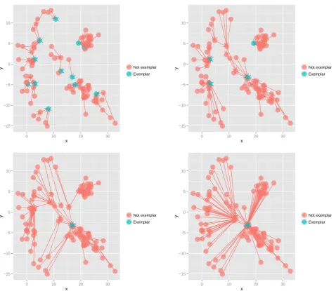
simulated dataset of Figure 1 (A). The dataset has

the 120 samples (n= 120). The four forests are

configured using the scale factors 5, 10, 20, and 40. The exemplars are displayed with a filled circle, they are the terminal nodes of the forests. The numbers of extracted exemplars are respectively equal to 8, 4, 2 and 1. Distinctly the number of exemplars depends on the

scale factork. The following describes the influence of

the scale factor.

2.5. Scale Factor

The higher the scale factor, the lower the number of exemplars. Moreover, when the scale factor increases

from one ton, the number of exemplars decreases from

nto one. Let us explain this property. Whenk= 1,N1(x)

is the singleton equal to x. Therefore each object x is

itself an exemplar ofΩ(i.e.xis linked tox). Then the

set of exemplars isΩ and the number of exemplars is

equal ton. Whenk=n,Nn(x) is equal toΩ. Each object

xis linked to the standard which has the highest DoR

withinΩ. Then the number of exemplars is equal to 1

the forest becomes only one tree and the standard is its

root. At the scalek, an exemplarxhas the highest DoR

within the neighborhoodNk(x) (i.e. within theknearest

neighbors ofx). Ifk1≤k2, thenNk1(x)⊆Nk2(x). Ifxis

an exemplar at the scalek2, then it is an exemplar at the

scalek1. Therefore the number of exemplars necessarily

decreases when the scale factor increases.

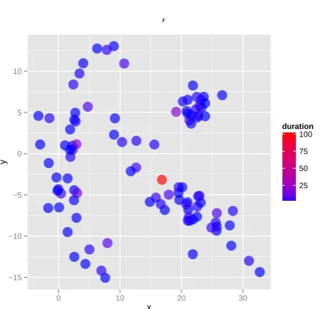
Increasing the scale factor, some exemplars could disappear among those who were extracted. But an object never appears as an exemplar if it was not

extracted at lower scale factor. Figure 4 displays the

duration of each exemplar when increasing the scale

factor. The exemplars are extracted from Figure 1

dataset (n= 100). When the scale factor is equal to 1,

all the objects are exemplars. When the scale factor increases, some exemplars disappear and their duration is shortened. Only the standard is kept from scale 1 to the scalen. It has the longest duration equal ton.

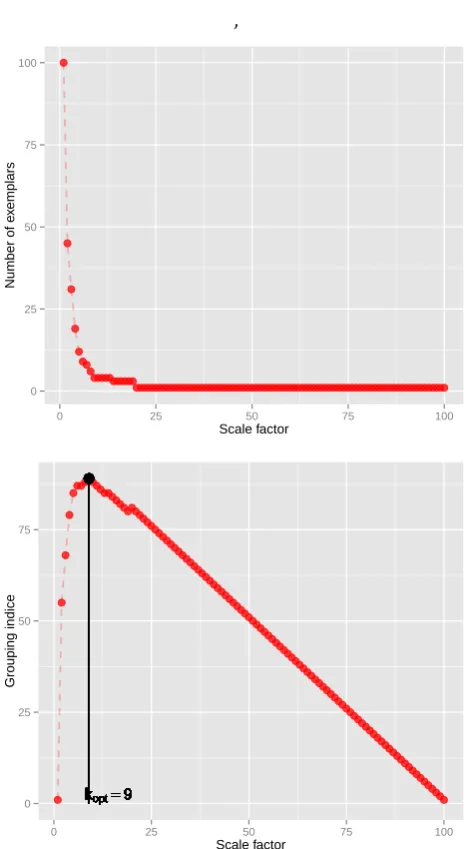
At the scale k, we assume that the numbers of

exemplars is smaller than n−₍_k−_{1) where} _k _{is the}

scale factor and n is the number of objects of the

dataset. At each scalek, we want to reduce the number

of exemplars. When this number is equal to n−_k₊

1, we consider that the extraction of exemplars is

suboptimal. This case is observed whenk= 1 ork=n.

In this paper, the scale factor becomes optimal when

the difference between n−_k_{+ 1 and the number of}

extracted exemplars is maximum. Let koptimum be this

optimal value of the scale factor we propose in this paper.

Figure5displays the numbers of exemplars according

to the scale factor k. It uses the dataset of Figure 1

(A) (n= 100). The scale factor increases from 1 to 100

and the number of exemplars decreases from 100 to

,

−15 −10 −5 0 5 10

0 10 20 30

x

y

25 50 75 100

duration

Figure 4. Duration of exemplars increasing the scale factor: The

Figure 1 dataset has 100 objects (n= 100). The scale factor increases from 1 (black) to 100 (red). When the scale factor is equal to 1, all the objects are exemplars. When the scale factor increases, some exemplars disappear. Only the standard is always extracted when increasing scale factor. Then its duration is equal to 100.

1. The numbers of exemplars is smaller than 101k.

The difference between 121−_k _{and the number of}

exemplars is maximum when k= 9. The black filled

circle shows this optimum value. Then four exemplars

are extracted usingk= 9.

3. Applications

This section presents applications of our method in two typical and very different contexts. The first application consists in extracting exemplars from a binary image database and building the graph of exemplars of this database. The second application present an analysis of the co-authoring in a research team by extracting exemplar authors and exhibiting the implicit structure.

3.1. Extraction of exemplars from a set of binary

images

In this first application we consider a set of binary images contained in a database. The goal is to extract exemplar images from this database. The interest could be providing a set of resuming images or distinguishing subsets of images according to their content. In a first step we construct the matrix of the relation by using

the Asymetric Haussdorff Distance. Classical methods

of clustering have to work with symmetric distance.

(6)

−15 −10 −5 0 5 10

0 10 20 30

x

y Not exemplar

Exemplar

−15 −10 −5 0 5 10

0 10 20 30

x

y Not exemplar

Exemplar

−15 −10 −5 0 5 10

0 10 20 30

x

y Not exemplar

Exemplar

−15 −10 −5 0 5 10

0 10 20 30

x

y Not exemplar

Exemplar

Figure 3. Networks obtained with scale factork= 5,k= 10,k= 20, andk= 40 with dataset of Figure1(A). The exemplars are

displayed with blue filled circles.

image A. As we wrote at the beginning of this paper, the symmetry property is not required in our method.

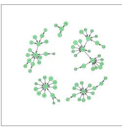
Firstly, we compute the score of each image of the database. In a second step we build the associated

directed graph presented in Figure6and representing

the exemplars network (with a scale factor of 4). This graph shows how the dataset is structured. We can observe that the connected components of this graph are grouping image according to the object they represent. The three images that have no successors in this network are the exemplars of this dataset and they provide a good summary of the whole dataset.

3.2. Exploration of co-authoring network

The second application of our concept deals with publication data inside a laboratory, a research team or any other group of researchers.

(7)

,

0 25 50 75 100

Scale factor

Number of e

x

emplars

kopt=9

0 25 50 75

0 25 50 75 100

Scale factor

Grouping indice

Figure 5. Number of Exemplars (top) from Figure1(A) dataset

and Scale Factor : The number of exemplar is smaller than

100−₍_k−₁₎ _where _k _{is the scale factor and} ₁₀₀ _{is the}

number of objects of the dataset. The grouping index (bottom) (the difference between 100−₍_k−₁₎ _{(gray line) and the number of}

extracted exemplars (red points)) is maximal when the scale factor is equal to 9 (black circle).

account of their publication activity.

The dataset we used is the set of publications of the

CReSTIC Laboratory (University of Reims, France) [18].

This information is extracted from the web site of the laboratory.

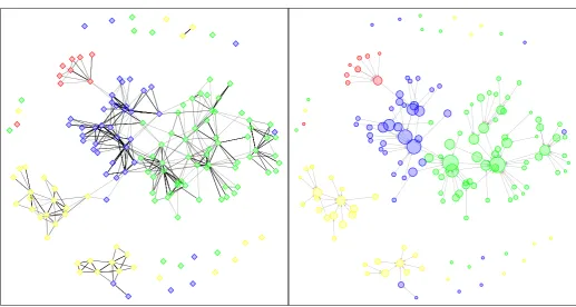
The graph of the Figure 7(Left) represents this

dataset. Each node is a lab member and each edge

between two members represents one common

publication. Different colors are used to represents

Figure 6. Network of the binary images where each image is

connected to one exemplar. This directed graph exhibits three connected components forming three clusters coinciding with the content of images

the different teams that compose the laboratory (but

this information is not used in the computation of the exemplars). Therefore the scale factor is not used in this application because the size of the neighborhood is implicitly fixed in the dataset (according to the number of co-author of each member of the team).

After computing the scores, we built the exemplars forest represented on the Figure7(Right). The size of the node is proportional to its score. This graph is displayed using the same position for the nodes.

The graphs presented in the Figure 7 show several

interests of our method. The first interests is the

sim-plification of the graph of the Figure7(Left). When the

numbers of vertices and edges are growing the graph becomes more unreadable. For big data, resuming and simplifying is a necessary task.

The second interest is to exhibit such a sub-structure of the team (this task is called community detection

in a network [19]). The Figure 7 (Right) shows how

groups are connected, and which members are the most representative. The exemplars members are connecting the others and can be viewed as natural leaders (or natural mentors) according to their publications and their co-authors. It emphasizes the important (critical) position of some members in a research team.

(8)

Figure 7. Left : Forest of the co-authoring in a laboratory. Each vertex is one researcher and each edge corresponds to one common publication. Right : Representative Network. The higher is the score of one researcher, the higher is the diameter of its vertex in the graph. In this graph, each edge is the link of one researcher to its exemplar.

components is a little bit different of the real partition-ing in sub-groups (represented by the different colors)

3.3. Structuration of a medical database

In this case study, we consider a dataset of 71 diabetic patients described by 10 variables. This dataset was constitued by the endocrinology service of the University Hospital Center (CHU) of Reims. Our goal is to exhibit how the medical cases could be linked. After computing the distance matrix between patients

with the Chebyshev distance [20], we obtain the forest

shown in the figure8according to the DoR of patients.

The resulting forest structures the raw database as a network of medical cases. We can see this graph as a knowledge representation extracted from data and could be view as a first step for building a medical case based reasoning system.

4. Conclusion

In the framework of data mining, this paper describes a new way for extracting exemplars from a relational dataset. The method we propose is based on a pairwise comparison assuming a coarse relation on the dataset. This approach is particularly adapted when no distance is available or meaningful in the data domain. Moreover the coarse relation between data does not

need symmetry or transitivity properties. Thus the method is useful for any kinds of relational data. The DoR is defined from these pairwise comparisons. The paper defines the standard which is the sample with the highest score. Simulations show the robustness of the standard against outliers and the stability of the standard when resampling dataset. Thus these results confirm the standard as a robust location estimator. Moreover the DoR is used to extract exemplars which are real objects. Then our approach of location estimator avoids the drawbacks of average objects which are meaningless when processing qualitative data.

Using a score based on the pairwise comparison, we define the k nearest neighbors of each datum. This approach permits us to extract exemplars depending on this k value. We state that the number of local exemplars decreases from n to 1 (n is the number of data samples) when k value increases from 1 to n. Thus k is considered as a scale factor. The method we propose allows us to explore the dataset through different scales. We can adjust the k value for extracting a reduced number of exemplars. An automated approach is proposed to determine an optimal number of exemplars.

(9)

1

2 3 4

5

6

7 8

9 10

11

12 13

14

15 16

17

18

19 20

21

22 23

24 25

26 27

28 29 30

31 32

33 34

35

36

37 38

39

40

41 42

43 44

45 46

47

48

49 50

51 52

53 54

55 56

57

58

59

60

61 62

63 64

65

66 67 68

69

70 71

Figure 8. Forest obtained on a medical dataset. Data are

diabetic (type 2) patients described by 10 features including age, sex, HBA1C, prescribed insulin, body mass index etc. Each vertex is a patient and the circle diameter is proportional to the DoR of the patient. The scale factor k is determined by the method proposed in the section2.5

The forest eases the explanation of the exemplar roles in the dataset. When the scale factor increases, some exemplars could disappear keeping the most important ones (i.e. the exemplars which are important nodes for connecting some data).

In future works we propose to use the fuzzy set theory

as in [21] to generalize our framework in the case of

fuzzy relation, when ranking data is not easy.

The major way we would to explore is the area of Social Network Analysis. We are convinced that our concept of exemplar could be a significant tool for extracting leaders or mentors in social network and improve recommendation systems. Our concept of degree of

representativeness should be compared to the different

definitions ofcentralityin a network [22].

References

[1] Frey, B. and Dueck, D. (2007) Clustering by passing messages between data points.Science315(5814): 972. [2] Pazzani, M. and Billsus, D. (2007) Content-Based

Recommendation Systems The Adaptive Web. In Brusilovsky, P., Kobsa, A. and Nejdl, W. [eds.] The Adaptive Web (Berlin, Heidelberg: Springer Berlin / Heidelberg), Lecture Notes in Computer Science 4321, chap. 10, 325–341. doi:10.1007/978-3-540-72079-9_10.

[3] Brun, A., Hamad, A.,Buffet, O. andBoyer, A.(2010) Towards preference relations in recommender systems. InECML/PKDD Workshop on Preference Learning (PL-10). [4] Newman, M.E.J. and Girvan, M. (2004) Finding and evaluating community structure in networks.Phys. Rev. E69: 026113. doi:10.1103/PhysRevE.69.026113. [5] Tuzhilin, A.(2012) Customer relationship management

and web mining: the next frontier. Data Mining and Knowledge Discovery: 1–29.

[6] Alfred, R. (2010) Summarizing relational data using semi-supervised genetic algorithm-based clustering techniques.Journal of Computer Science6(7): 775–784. [7] Jain, A.K., Murty, M.N. and Flynn, P.J. (1999) Data

clustering: a review.ACM Computing Surveys31(3): 264– 323.

[8] Lühr, S.andLazarescu, M.(2008) Connectivity based stream clustering using localised density exemplars. In Proceedings of the 12th Pacific-Asia conference on Advances in knowledge discovery and data mining, PAKDD’08 (Berlin, Heidelberg: Springer-Verlag): 662–672.

[9] de Borda, J.C. (1781) Mémoire sur les élections au scrutin.Mémoires de l’Académie Royale des Sciences: 657– 664.

[10] Barnett, V. (1976) The ordering of multivariate data. Journal of the Royal Statistical Society, Series A (General)

139(3): 318–355.

[11] Conover, W.J.andIman, R.L.(1981) Rank transforma-tions as a bridge between parametric and nonparametric statistics.The American Statistician35(3): 124–129. [12] David, H.A.andNagaraja, H.N.(2003)Order Statistics

(Wiley), 3rd ed.

[13] van Erp, M. and Schomaker, L. (2000) Variants Of The Borda Count Method For Combining Ranked Classifier Hypotheses. InSeventh International Workshop on Frontiers in Handwriting Recognition: 443–452. [14] Thomas, G.E. (2000) Use of the bootstrap in robust

estimation of location.The Statictician49(1): 63–77. [15] Rousseeuw, P.J.andLeRoy, A.M. (2003)Robust

Regres-sion and Outlier Detection(Wiley).

[16] Mcgovern, A., Friedl, L., Hay, M., Gallagher, B., Fast, A., Neville, J. and Jensen, D.(2003) Exploiting relational structure to understand publication patterns in high-energy physics.SIGKDD Explorations5: 2003. [17] Neville, J.,Adler, M.andJensen, D.(2003) Clustering

relational data using attribute and link information. In Proceedings of the Text Mining and Link Analysis Workshop, 18th International Joint Conference on Artificial Intelligence: 9–15.

[18] Benassarou, A.andCutrona, J.(2010), Crestic publica-tion database. URLhttp://crestic.univ-reims.fr/. [19] Papadopoulos, A., Lyritsis, A. andManolopoulos, Y.

(2008) SkyGraph: an algorithm for important subgraph discovery in relational graphs. Data Mining and Knowledge Discovery17(1): 57–76. doi: 10.1007/s10618-008-0109-y.

[20] Abello, J., Pardalos, P.M.andResende, M.G.C. [eds.] (2002)Handbook of Massive Data Sets(Norwell, MA, USA: Kluwer Academic Publishers).

(10)