Generalized Encoding CRDSA: Maximizing Throughput in Enhanced Random Access Schemes for Satellite

(1)

Generalized Encoding CRDSA: Maximizing

Throughput in Enhanced Random Access Schemes

for Satellite

Manlio Bacco

12,∗

, Pietro Cassará

1

, Alberto Gotta

1

1_{National Research Council of Italy (CNR), Institute of Information Science and Technologies (ISTI)} 2_{University of Siena, Information Engineering and Mathematic Science Department}

Abstract

This work starts from the analysis of the literature about the Random Access protocols with contention resolution, such as Contention Resolution Diversity Slotted Aloha (CRDSA), and introduces a possible enhancement, named Generalized Encoding Contention Resolution Diversity Slotted Aloha (GE-CRDSA). The GE-CRDSA aims at improving the aggregated throughput when the system load is less than 50%, playing on the opportunity of transmitting an optimal combination of information and parity packets frame by frame.

This paper shows the improvement in terms of throughput, by performing traffic estimation and adaptive

choice of information and parity rates, when a satellite network undergoes a variable traffic load profile.

Keywords: Satellite, Interference Cancellation, DVB-RCS2, CRDSA, Slotted Aloha, Random Access

1. Introduction

Satellite access networks provide a wide range of services for civil and military applications. These services include mobile data transfer, localization, satellite television and Internet web traffic. The Second Generation DVB Interactive Satellite Services (DVB-RCS2) [? ] was recently introduced as a renewed standard for satellite communications and is specifically designed for Internet based services. Internet traffic is highly dominated by short-lived connections [?] and message exchanges, as far as mobile applications have gained the largest part of the Internet share. As shown in [? ], the performance of access scheme are strongly linked to the traffic characteristics and in particular to the size of the file transferred. In addition, the advent of IoT (Internet of Things) services is boosting the bursty nature of the Internet traffic: such an evolution of the traffic nature requires adequate measurements on the multiple access protocols, in order to settle the suitability of either a Random Access (RA) or a Dedicated Access (DA). In this paper, a study on a generalized case of a Coded Slotted Aloha (CSA) is presented, showing that the random choice of information and redundancy lengths can improve the performance, in terms of throughput. In particular, runned simulations show that the design of a load control mechanism can help in obtaining a reasonable

level of performances per load level, avoiding the complexity of a DA-like approach.

The rest of the paper is organized as follows: an highlight on the most relevant related works on Slotted Aloha (SA) based access protocols is presented in Section??. In Section??, the load estimation strategy is shown, as well as an ideal load control strategy based on Cross Entropy (CE) theory. The major contribution of this work is in Section??, a simple but efficient load control strategy that works without an a priori heuristic and guarantees a clear performance gain. Section ?? shows the results of the simulations, where the two control strategy are compared. Finally, the conclusions are in Section??.

2. Related Work

Many efforts have been made in the field of random access protocols for satellite communications, aiming at maximizing the aggregated throughput. Contention Resolution Diversity Slotted Aloha (CRDSA) [? ] has been introduced in DVB-RCS2 standard [? ] for data traffic with a dedicated system profile for SCADA (Supervisory Control And Data Acquisition) and M2M (Machine to Machine) communications. The advantage of contention resolution is represented by the increment of the performance in terms of throughput. In fact, CRDSA exhibits almost ideal performances (i.e low collision losses), up to 50-60% of the global access

Research

Article

EAI Endorsed Transactions

on

Mobile

Communications

and

Applications

Receivedon 13 February 2014;acceptedon 24 September 2014;publishedon 28 December 2014

Copyright© 2014 Manlio Bacco et al.,licensedtoICST.Thisisanopen accessarticledistributedunderthetermsofthe Creative Commons Attribution license (http://creativecommons.org/licenses/by/3.0/), which permits unlimited use,distributionandreproductioninanymediumsolongastheoriginalworkisproperlycited.

(2)

CRDSA and SA assume the MAC frame duration equal toTF, during whichNs slots are allocated. The timeslot

has a duration of TS =TF/Ns. Assuming that in each

frame u users try to access the shared channel, each user transmits one or more replicas of the same packet in the current MAC frame. In each packet a pointer to the positions of its replicas is included. The pointer is used to locate its own other replicas into the frame and to remove the interfering ones in the collided slots. The contention resolution proceeds iteratively, by removing the decoded signals in the relative collided slots. At the end of the procedure the Packet Loss (PL) due to

the un-cancelled collisions is significantly reduced. By definition, the throughput is given by:

T =G(1−_P_L_), ₍₁₎

where G=_Nu

s is the number of packet transmission

attempts per frame, i.e., the load of the system, when a single information packet is transmitted per user per frame. In SA, (1−_P_L_{) is the probability that no} others attempts of transmission arises during a timeslot. This value can be calculated through the Poisson distribution:

P(k) =Gke

−_G

k!

at k= 0. Let G∗ be the supremum of G such that, in the asymptotic settingu→ ∞_{, the throughput}_T _fulfills T =G; thereforeG∗is the asymptotic peak throughput. In SA, the maximum throughput T_SAmax=G∗e−G∗ = 1_e, is achieved for G∗= 1. When CRDSA operates at a given G, reducing PL leads to a throughput gain with

respect to SA and its non-SIC variants, as in DSA [? ] with two or more replicas for each information packet transmission. This improvement is quantified in [? ] as the normalized throughput TCRDSA≈0.55, which

is the probability of successful packet transmission per timeslot, whereas the peak throughput for SA is TSA≈ 1e . Further improvements can be achieved by

exploiting the capture effect [? ] [? ]. In [? ] Irregular Repetition Slotted ALOHA (IRSA) was introduced to provide a further throughput gain over CRDSA. Higher throughput can be achieved by IRSA, allowing the Satellite Terminal (ST) to choose the number of replicas in a random way. As stated in [? ], both CRDSA with one replica and CRDSA++ with more replicas can be considered as particular cases of IRSA where the repetition rate, frame by frame, is fixed. In [? ], it is shown that a variable repetition rate does not introduce significant improvements in terms of throughput, if the set of slots per frameNsis limited to about a hundred of

slots, that is the range foreseen in DVB-RCS2 standard [?]. In [?], the throughput TIRSA≤0.8, but Ns ranges

up to 200 slots.

While CRDSA, CRDSA++ and IRSA are based on repetitions, Coded Slotted ALOHA (CSA) encodes an information burst - multiple of a timeslot - prior transmitting [?].

All the protocols so far discussed implicitly impose that the average load in the system is targeted around the G∗

value. Otherwise, no improvement is appreciable. A centralised load control should estimate the current system load and dynamically reduce or increase the allocated set of slot Ns, by adapting the

frame duration. Since Ns in DVB-RCS2 standard is

bounded between 64 and 128 slots [? ], the satellite system may perform at G loads under the desired G∗, leading to the under-utilization of the available bandwidth. In CSA, the transmitted burst is made up of k= 2 information packets out ofntransmitted packets. The others n−_k _{packets are generated by a} packet-oriented binary linear block code.

Differently, a generalized case of CSA is presented in this work, named Generalized Encoding CRDSA (GE-CRDSA), where each ST randomly sorts the couple (n, k). Note that n=r+k, where r is the number of parity packets. GE-CRDSA aims at optimizing CSA, by allowing each ST to transmit more than two information packets per frame, leading in most cases to reduce the queuing delay with respect to those systems, which consider only a single information packet per frame.

3. Problem Definition and System Overview

Let us consider a SA system, with a MAC frame duration TF, composed ofNsslots. Letuibe a Poisson distributed

r.v. with meanG, which represents the number of active user terminals in frame i, being G the system load. In any frame, the ST randomly draws, over the set of C coding schemes, one couple (n, k), according to the Probability Mass Function (PMF) defined by the polynomial:

Ω(n,k)(x, y),

X

c

ωcxkcync, (2)

where the weight ωc is the probability of having kc

information packets over a nc-long codeword, for the

c-th coding scheme.

(3)

3.1. Load Estimation

Load Estimation (LE) techniques in [? ] estimates the probability that a slot is in a given state by using the binomial distribution theory. In order to estimate the offered traffic load, a slot state can be in idle (I), successful (S) or collided (C) state, which represent zero, one or two (or more) bursts transmitted in aTs,

respectively. In SA, given the normalized offered loadG and the frame lengthNs, the expected numbers of slots

per state per frame is defined in [?] as:

sI(G, Ns) =Ns(1−p)GNs, (3)

sS(G, Ns) =GNs(1−p)GNs

−₁

, (4)

sC(G, Ns) =Ns−sI−sS, (5)

whereGNs is the number of bursts per frame andp=

1/Ns is the probability that the burst of a single node is

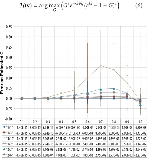
in a given slot. The LE techniques asses the estimated offered load ˆGby inversely tracking equations (??)-(??) from the observed vectorv= {i,s,c}, wherei,s, andcare the number of slots per frame in the I, S, and C states, respectively. Let H _{be an LE function that returns ˆ}_G, which are given in [?] by:

H₍_v_{) = arg max}

G

Gse−GNs_(eG−₁−_G)c ₍₆₎

0.1 0.2 0.3 0.4 0.5 0.6 0.7 0.8 0.9 1.0 "1/1" -1.40E-15 -3.00E-15 5.94E-15 -6.00E-15 0.00E+00 -6.00E-04 -2.00E-03 -1.50E-03 1.10E-03 -6.80E-03 "1/3" -1.40E-15 -3.00E-15 5.94E-15 -6.00E-15 2.10E-03 6.00E-03 8.50E-03 8.80E-03 9.90E-03 -1.43E-02 "5/10" -1.40E-15 -3.00E-15 5.00E-03 2.36E-02 3.99E-02 9.99E-02 1.59E-01 1.39E-01 7.59E-02 -1.22E-02 "1/2" -1.40E-15 -3.00E-15 5.94E-15 -6.00E-15 -1.00E-04 2.40E-03 5.40E-03 6.10E-03 3.50E-03 -1.44E-02 "3/7" -1.40E-15 -3.00E-15 1.10E-03 7.80E-03 1.71E-02 2.74E-02 4.49E-02 4.89E-02 2.54E-02 -2.94E-02 "2/6" -1.40E-15 -3.00E-15 1.00E-04 4.00E-03 1.28E-02 1.85E-02 2.75E-02 2.93E-02 2.06E-02 -2.23E-02

-0.10 -0.05 0.00 0.05 0.10 0.15 0.20 0.25 0.30 0.35

Error on Estimated G

!

Load G!

Figure 1. Error on load estimation (Ns=100) by using LE

techniques combined with the use of linear codes in transmission. Codes in the table are in the form(k, n).

In order to apply Eq. (??) in CSA and therefore in GE-CRDSA, you must divide the return value of H by n, because the physical load is increased by the

code length. Therefore, the process of dividing the load estimation by n leads to an estimation of the offered load. In order to obtain the normalized offered load Gest, the estimated offered load must be divided by

the number of the timeslots Ns. Figure ?? shows the

simulation results of Eq. (??) with different coding schemes, whenNs = 100. The error on load estimation

is visible, together with the 0.05, the 0.50 and the 0.95 quantiles of the values collected during a Montecarlo test session. You can also read plot value in the table below the figure, where linear codes are presented as k/n in the first column. It is visible as, when using a linear code with k >1, the estimation is subject to an increasing error.

3.2. Cross Entropy Control Strategy

In order to define a control law to extract the couple (n, k) at the G value that maximizes the aggregated throughputT, the controller needs either the a priori information, as the heuristic shown in Table ??, or an analytical model as in [?], which provides the average throughput as a function of G, k and n. It is worth noting that a closed analytical form to derive the packet loss (or the throughput) value, given the parametersNs,

k,nandGis still absent, as far as the authors know. Assuming that any station, in framef, can randomly choose the couple (n, k) according to the PMFΩ(n,k), the

throughput maximization over all the possible couples (n, k) can be formally stated as:

max{_T}_Ω (n,k)

s.t. k≤_k_max n≤_n_max PL≤θ

(7)

G (n,k) T PL

0.1 (10, 5) 0.460 6.598e−02 0.2 (7, 3) 0.527 1.222e−01 0.3 (6, 2) 0.586 3.288e−02 0.4 (4, 1) 0.400 5.00e−05 0.5 (4, 1) 0.500 1.23e−03 0.6 (3, 1) 0.600 2.93e−₀₂

0.7 (3, 1) 0.676 2.952e−₀₂

0.8 (3, 1) 0.536 3.083e−01

0.9 (2, 1) 0.425 5.319e−01 1.0 (2, 1) 0.373 6.361e−01

(4)

The solution of the optimization problem (??) is given by the PMF Ω(n,k), used by the ST to draw the

number of information and redundancy packets to be transmitted in the next frame f. The constraints of the optimization problem are the maximum allowed number of information packets k and the maximum number of packetsn1_{per station per frame and, finally,} the maximum value of PL that can be tolerated. This

problem can be addressed through the approaches either analytical or numerical [? ]. Note that the first approach gives much more information about the behavior of the system.

In [?] an exhaustive evaluation of the possible couples (n, k) is presented, in order to achieve the maximum aggregated throughput, when Ns ranges from 100 to

1000 slots. For practical reasons, the main interest is for theNsrange foreseen in DVB-RCS2. Table??shows

the optimal choice of the couple (n, k) that achieves the maximum aggregated throughput whenNs=100 andG

ranges between 0.1 to 1.

Note that the load estimation may be defected by an estimation error, as shown in Figure??. In addition, the satellite feedback delay makes the estimation obsolete at least of the satellite latency (more than 250ms). As shown in [? ] and [? ], IRSA and CSA protocols can have enhancement in their performance, if a variable repetition rate is used. Note that, the G∗ tracking problem is not trivial because the error estimation may lead the system to operate in the rangeG >0.7, where it is deeply unstable and the collision rate is the prevailing factor in channel rate under-utilization.

Next it is shown how the problem discussed so far can be addressed by an iterative algorithm based on the Cross-Entropy theory. In the proposed formulation, it is assumed that C is the finite set of available coding schemes (n, k). Moreover, it is assumed that the c-th coding scheme holds the probability to be drawnωc.

The problem can be stated as follows: finding the PMFΩ_(n,k)of the coding schemes, which maximizes the objective function OT((n, k)) given by the aggregated

average throughput T, assuming that the aggregated average packet loss probability PL is within a given

range.

The approach discussed in this section explores the space of solutions by a random method. Let γ be the maximum value of the objective function for the optimal couple (n, k)opt_{. To solve the stated}

problem the PMF Ωopt_(n,k) must be identified over the optimization domain. Hence our optimization problem can be viewed also as the maximization probability that our objective function is greater than γ over all the possible solutions for the PMFΩ_(n,k):

1_{Note that, in case of a single terminal, it would be possible that}

k≤_n_max≤_N_s, i.e., the station utilizes the entire frame.

PΩ₍_n,k₎{OT((n, k))≥γ}=EΩ₍_n,k₎

n I_O

T((n,k))≥γ

o . (8)

The weightsωcable to maximize the probability of the

eventO_T((n, k))≥_γ_{in Eq. (}_??_{) must be estimated.} This problem can be viewed as a Stochastic Node Network (SNN) problem with a set of nodes{_1,· · ·_{, U}} and a set of node characteristics {_1,· · ·_{, C}}_distributed according to Ω_(n,k). The objective is to assign the node characteristics following Ω_(n,k) in a way that the objective function is maximized. Assuming that the nodes of the network sort the coding scheme independently andωcis the probability for the couplec

to be drawn, the vectorΩ={_ω₁_,· · ·_{, ω}_C}_{represent the} PMF from which any node draws its coding scheme.

This kind of SNN problems can be resolved through the Cross-Entropy (CE) method using an algorithm. The solution relies on the steps shown in Algorithm??.

Algorithm 1Optimal PMF Algorithm

1. Generate the initial distributionΩ0= [ ˆω (0) 1 ,· · ·,ωˆ

(0)

C ]

with entriesωˆ(0)c = _C1;

whileDKL

ˆ

Ω(t)_(n,k),Ωˆ(t_(n,k)−1)

≥_do

2. Generate S random vectors {_{(n, k)}1_s· · ·_{(n, k)}u_s}_; _s₌ 1· · ·_S _{of the} _u _{coding schemes used by the} _u _users {_{(n, k)}1_s · · ·_{(n, k)}u_s} ∼_Ωˆ(t−1)

(n,k);

3. Evaluate the (1-α)-quantile of the sample coding schemes, for which the objective function is greater thanγˆ(t−1)_;

4. Update the estimation Ωˆ(t_(n,k)−1) to Ωˆ(t)_(n,k)((n, k)) through the samples that belong to the (1-α)-quantile 5. Evaluate the KL-Distance between the Mass Probability Functions at(t)and(t−₁₎

t=t+1

end while

The (1−_{α)-quantile ˆ}_γ(t)_{of the estimated PMF ˆ}Ω(t)_(n,k)

can be evaluated through Eq. (??).

ˆ γ= max

o|_P_ˆ

Ω(n,k)(OT((n, k))≥o)≥α

. (9)

The evaluation of the Kullback-Leibler distance (KL-Distance) between ˆΩ(t)_(n,k)and ˆΩ(t_(n,k)−1)at the step (5) of the Algorithm??can be evaluated as follows:

DKL( ˆΩ (t) (n,k),Ωˆ

(t−₁₎

(n,k)) =

X

U

ˆ

ω(tc−1)log

       ˆ ω(t)c

       . (10) ωˆ(ct

(5)

The KL-Distance measures how much the new PMF is different from the previous one.

The update of the estimation ˆΩ(t_(n,k)−1)at step (4) by the selected sample can be performed by the Eq. (??):

ˆ ω(t)c =

S

X

s=1

I_{

OT((n,k)s)≥γˆ(t)}I{ωc}

S

X

s=1

I_{

OT((n,k)s)≥γˆ(t)}

. (11)

This equation shows that the weights of the new PMF are the occurrences of the coding scheme of the samples belonging to the (1−_α_)-quantile.

To amplify the CE selection of the weights of the PMF, the entries of the estimated ˆΩ(t)_(n,k) are modulated as in the Eq. (??).

ˆ ω(t)c =

                                   ˆ ω(tc−1)

                  

1 + _CT((n, k)c) X

c=1

T((n, k)c)

                  

,c∈_S_best

(1−

C

X

c=1

ˆ

ω(tc−1)) ˆω(t

−₁₎

c ,c<Sbest,c

0_∈

Sbest

(12)

In Eq. (??), Sbest is the set of coding scheme samples

belonging to the (1−_{α)-quantile. The first row shows} how the weights of the coding schemes belonging to the Sbestare increased proportionally with the increment of

throughput given to these coding schemes. Instead, the second row shows how the other weights are decreased proportionally, in a way that the new PMF does not change abruptly w.r.t. the previous one.

3.3. Load Control Strategy

In this section a different technique is presented, with respect to the one described in section??. The idea is to find a control algorithm able to perform, at least, as the one based on Cross-Entropy theory, while removing the need for an heuristic, i.e., for a priori known data.

This Load Control (LC) strategy is applied to the described system, in order to maximise the throughput T, given the estimated loadG, computed as described in section??. Given thatuusers access to the channel at the same time using the same PMF, the aggregated mean value (n, k) and the code selection probabilityωc, used

by the Satellite Terminals (ST s), can be evaluated. In order to control and to bind the packet lossPLperceived

by the ST s, an observer-like technique is exploited, using a window-based algorithm. The decoding process

of the frame provides information to the observer about the coding scheme, the local throughput and the packet loss of theST s. By taking advantage of this information, the statistics computed by using the collected data can be used to control the performance of the system.

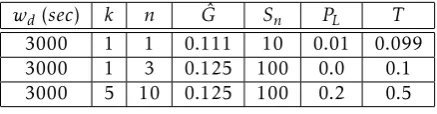
Table??shows the structure of the typical observation window. In the first column of the table, the time window duration wd= (te−ts) is shown, where ts and

teare the timestamps representing the start and the end

time of the window. The remaining columns show the transmitted information lengthk, the code lengthn, the estimated load ˆG, the number of collected samplesSn

within the window for the given coding scheme (i.e., the number ofST s that have transmitted duringwd using

that linear code). The last two columns show the values of PL and T for that specific linear code, in terms of

mean value, given the number of samplesSn. Note that

the single window can be viewed as a set of tuples of cardinality equal to the number of different linear codes that eachST can use during the transmission.

wd(sec) k n Gˆ Sn PL T

3000 1 1 0.111 10 0.01 0.099

3000 1 3 0.125 100 0.0 0.1

3000 5 10 0.125 100 0.2 0.5

Table 2. Sample data from an observation window.

The proposed control algorithm periodically analyzes the last available window, with a period ofLCpseconds,

in order to determine the aggregated mean value (n, k) and the correspondingPL of the system. The controller

will shift the (n, k) value, by changing the weights of the PMFΩ(n,k), in order to improve the performances.

The main idea behind this control algorithm is to target a given PL in the shortest possible time.PL can

be reduced by increasing the probability of drawing a code that fosters thePL closer to the chosen packet loss

value. For instance, referring to Table??and assuming the target PL = 0.18, the aggregated packet loss can

be forced to a value close to the PL of the last row,

increasing the probability to select the code (n, k) = (nc, kc) = (10,5), where (nc, kc) is the code (or the code

set) that ensures the target will be reached as quickly as possible.

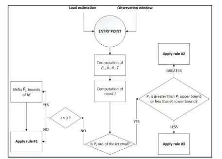
The controller periodically acts as described in Figure ??: it receives as input the estimated load and the last available observation window. These data are used to estimatePL, (n, k) andT.

Let T(i) and P_L(i) be the throughput and the packet loss, respectively, at time ti. Tmax represents the

(6)

Figure 2. Load Control Algorithm flowchart - the rules are detailed in Algorithm??

J =sgn((Tmax−T(i)))|(Tmax−T(i))−(P (i)

L −P

(i−₁₎

L )|

(13)

This formulation ensures thatJ is strictly positive only if the T is increasing and its value depends on the difference between (T(i)₋_T(i−₁₎

) and (P_L(i)−_P(i−1)

L ). The

so-calledtrend is a metric used to evaluate the system behavior; ifJ >0, the system is performing better than in the previous time window. The target PL is upper

and lower bounded by the values PL(up) and PL(lo),

respectively, given thatPL(up)−PL(lo)>0.

The target Packet Loss is defined as follows:

PL(target)= (PL(up)−PL(lo))/2. (14)

The distancedbetween the current packet lossPL and

the target packet lossPL(target), defined as:

d=|_P_L(target)−_P_L| ₍₁₅₎

is used in the calculation of the coefficient g= 0.5d. The control algorithm adds g to the weight of the selected linear codes and accordingly reduces the other weights. The increment grows linearly with d. Hence,

the PL(target) can be quickly reached. The maximum

value ofg is 0.5, which means an increment of 50% for the extraction probability of the corresponding coding scheme ford= 1.

Referring to Figure ??, the algorithm estimates PL

and T using the last available observation window. ThenJis computed. Given the current load level, when J >0 and PL(up)≤PL≤PL(lo), only one of the following

conditions is verified in the previous time window: (i) the throughput gain is higher than the packet loss gain; (ii) the packet loss reduction is higher than the throughput reduction; (iii) the throughput has been increased and the packet loss has been reduced. This leads to shift up PL(up) and PL(lo). The bounds are

redefined as: PL(lo)=PL(lo)+M and PL(up)=PL(up)+M,

whereMis a tuning factor reported in Table??.

The selected codes (nc, kc) are the ones able to quickly

target the desired value of packet loss: PL(target). The

(7)

system behavior, as well as from the results presented in the section??.

Algorithm 2Load Control Algorithm

if{_P_L(lo)≤_P_L≤_P_L(up)}_then

(RULE #1)

ωj =ωj+f; j= (nc, kc−1)

ωi =ωi+f; i= (n_k(kc+ 1), kc+ 1)

(n, k)≈_(n_c_{, k}_c₎

subject to:2kc≤nc≤4kc

else if{_P_L≥_P_L(up)}_then (RULE #2)

ωj =ωj+f; j= (kc, nc)

kc= min{(k−(k−kmin)∗d, kmin)}

ifkc,kminthen

nc= (n/k)∗kc

else

nc= max (nc−1, nmin)

end if subject to:

ifGest ≤Gpeakthen

3kc≤nc≤4kc

else

2kc≤nc≤4kc

end if

else if{_P_L≤_P_L(up)}_then (RULE #3)

kc= min (kc+ 1, kmax)

nc= (n/k)∗kc

subject to:2kc≤nc≤4kc

end if

The choice for the numerical values used with the Algorithm??is detailed in Table??.

Description Parameter Value

Min info size kmin 1

Max info size kmax 10

Min code length nmin 1

Max code length nmax 15

LC chosenk kc [kmin, kmax]

LC chosenn nc [nmin, nmax]

Gpeak threshold Gpeak 0.80

PLtuning factor M 0.005

InitialPL(up)value PL(up) 0.03

InitialPL(lo)value PL(lo) 0.01

Ωiatt=0 Ω0i 1/length(C)

Control interval LCp 3s

Window duration wd 3s

Table 3. Simulation and tuning parameters for the LC algorithm

4. Numerical Results

The previous section describes the mathematical framework behind the GE-CRDSA. The algorithm allows the users to randomly choose the number of information and parity packets by using the PMFΩ_(n,k). In this section, by exploiting the simulation results, it is shown how the PMF, and consequently the choice of (nc, kc), affects the throughput and the packet loss for

differentGvalues.

An ad-hoc simulator has been developed to test the two algorithms. The system and simulation parameters for the satellite scenario are summarized in Table??.

Parameter Value

Bandwidth 8 Mhz

Modulation QPSK

Phy FEC 1/3

Frame Duration 0.026s

Ns(slots) 100

IC max iterations2 20

Table 4. Simulation parameters for the case study

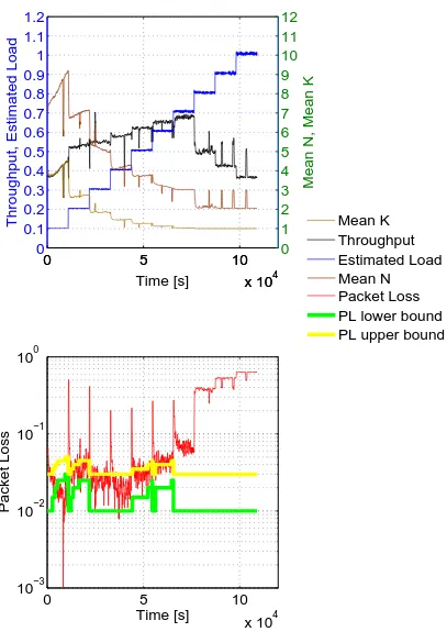
The simulation results are here presented. The LC technique and CE control strategy are compared, initially by forcing them to use the same set of linear codes C, detailed in table ??. Figures ?? and ?? show the case of increasing G, while Figures ?? and ?? the decreasing one. A randomGfluctuation can be obtained from those two profiles. In fact, a realGprofile usually exhibits slower variations than those presented here. It is worth noting that the LC outperforms that based on CE theory in terms of throughput atGbetween 0.6 and 0.4, while the two control techniques show comparable behaviors at other loads.

In Figure ??, throughput and packet loss are shown for a larger set of codesC, upper bounded bynmaxand

kmax, as in Table ??. In fact, the LC technique is not

limited by an a priori information request. Therefore whateverC is, it slowly adjusts theΩin the described way. On the other hand, the CE Control Strategy (CECS) offers the possibility to immediately use theΩshowing the highest throughput at thatGvalue, because of the heuristic. The LC and CE algorithms use a different codes distribution at each load level. If you refer to (n, k) plots, it is possible to see how the same throughput value can be reached using a different PMF. In Figure ??, it is also possible to view PL(up) and PL(low) values

and how thePLvalue is bounded within, forGfrom 0.7

2_{The interference cancellation (IC) process performs several}

(8)

0

0.5

1

1.5

2 x 10

4

0

0.1

0.2

0.3

0.4

0.5

0.6

0.7

0.8

0.9

1

1.1

1.2 Time [s]

Throughput, Estimated Load

0

0.5

1

1.5

2 x 10

4

0

1

2

3

4

5

6

7

8

9

10

11

12

13

14

15

16 Mean N, Mean K

0

0.5

1

1.5

2 x 10

4

10

−3

10

−2

10

−1

10

0

Time [s]

Packet Loss

Throughput

Estimated Load

Mean N

Mean K

Throughput

Estimated Load

(9)

0

5

10 x 10

4

0

0.1

0.2

0.3

0.4

0.5

0.6

0.7

0.8

0.9

1

1.1

1.2 Time [s]

Throughput, Estimated Load

0

5

10 x 10

4

0

1

2

3

4

5

6

7

8

9

10

11

12 Mean N, Mean K

0

5

10 x 10

4

10

−3

10

−2

10

−1

10

0

Time [s]

Packet Loss

Throughput

Estimated Load

Mean N

Mean K

Throughput

Estimated Load

Packet Loss

PL lower bound

PL upper bound

(10)

0

0.5

1

1.5

2 x 10

4

0

0.1

0.2

0.3

0.4

0.5

0.6

0.7

0.8

0.9

1

1.1

1.2 Time [s]

Throughput, Estimated Load

0

0.5

1

1.5

2 x 10

4

0

1

2

3

4

5

6

7

8

9

10

11

12

13

14

15

16 Mean N, Mean K

0

0.5

1

1.5

2 x 10

4

10

−3

10

−2

10

−1

10

0

Time [s]

Packet Loss

Throughput

Estimated Load

Mean N

Mean K

Throughput

Estimated Load

Packet Loss

(11)

0

5

10 x 10

4

0

0.1

0.2

0.3

0.4

0.5

0.6

0.7

0.8

0.9

1

1.1

1.2 Time [s]

Throughput, Estimated Load

0

5

10 x 10

4

0

1

2

3

4

5

6

7

8

9

10

11

12

13

14

15

16 Mean N, Mean K

0

5

10 x 10

4

10

−3

10

−2

10

−1

10

0

Time [s]

Packet Loss

Throughput

Estimated Load

Mean N

Mean K

Throughput

Estimated Load

Packet Loss

PL lower bound

PL upper bound

(12)

0

5

10

15 x 10

4

0

0.1

0.2

0.3

0.4

0.5

0.6

0.7

0.8

0.9

1

1.1

1.2 Time [s]

Throughput, Estimated Load

0

5

10

15 x 10

4

0

1

2

3

4

5

6

7

8

9

10

11

12

13

14

15

16 Mean N, Mean K

0

5

10

15 x 10

4

10

−3

10

−2

10

−1

10

0

Time [s]

Packet Loss

Throughput

Estimated Load

Mean N

Mean K

Throughput

Estimated Load

Packet Loss

PL lower bound

PL upper bound

(13)

0 0.1 0.2 0.3 0.4 0.5 0.6 0.7 0.8 0.9 1

linear codes set

PMF

1,1 2,1 3,1 4,1 5,1 6,1 7,1 8,1 9,1 _10,1 2,2 3,2 4,2 5,2 6,2 7,2 8,2 9,2 _10,2 3,3 4,3 5,3 6,3 7,3 8,3 9,3 _10,3 _11,3 _12,3 4,4 5,4 6,4 7,4 8,4 9,4 _10,4 _11,4 _12,4 _16,4 5,5 6,5 7,5 8,5 9,5 _10,5 _11,5 _12,5 _13,5 _14,5 _15,5 6,6 7,6

estimated normalized load ~= 0.1 estimated normalized load ~= 0.2 estimated normalized load ~= 0.3 estimated normalized load ~= 0.4 estimated normalized load ~= 0.5 estimated normalized load ~= 0.6 estimated normalized load ~= 0.7 estimated normalized load ~= 0.8 estimated normalized load ~= 0.9 estimated normalized load ~= 1

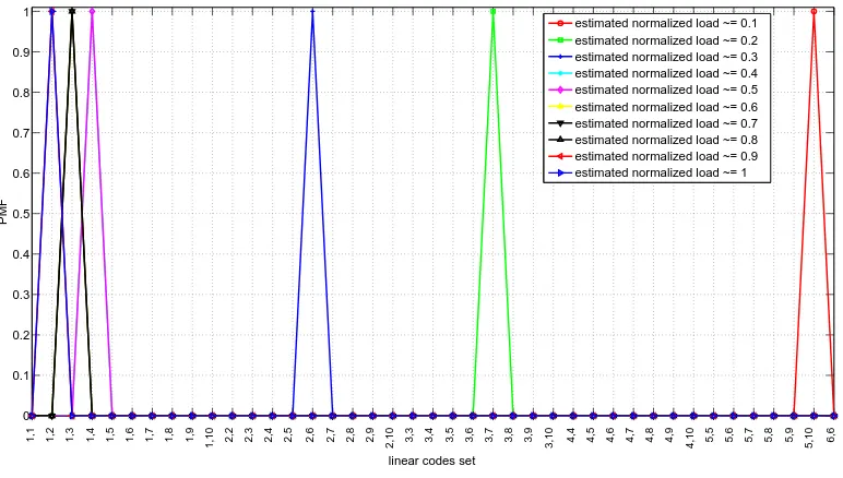
Figure 8. PMF for LC algorithm at different load levels for decreasingG, linear code setC as in table??.

0 0.1 0.2 0.3 0.4 0.5 0.6 0.7 0.8 0.9 1

linear codes set

1,1 1,2 1,3 1,4 1,5 1,6 1,7 1,8 1,9 _1,10 2,2 2,3 2,4 2,5 2,6 2,7 2,8 2,9 _2,10 3,3 3,4 3,5 3,6 3,7 3,8 3,9 _3,10 4,4 4,5 4,6 4,7 4,8 4,9 _4,10 5,5 5,6 5,7 5,8 5,9 _5,10 6,6

PMF

Figure 9. PMF for CE algorithm at different load levels for decreasingG, linear code setC as in table??.

to 0.1. ThePL bounds are shifted up in certain points,

according to the algorithm described in section??.

Figure ?? plots the PMF of the codes that produce the highest throughput in Figure ?? (i.e., at the time instant immediately before aGvariation), while Figure ??shows the PMF of codes when the CECS is selected.

Table??analytically describes the values of the PMF for the CECS.

(14)

0

5

10

15 x 10

4

0

0.1

0.2

0.3

0.4

0.5

0.6

0.7

0.8

0.9

1

1.1

1.2 Time [s]

Throughput, Estimated Load

0

5

10

15 x 10

4

0

1

2

3

4

5

6

7

8

9

10

11

12 Mean N, Mean K

0

5

10

15 x 10

4

10

−3

10

−2

10

−1

10

0

Time [s]

Packet Loss

Throughput

Estimated Load

Mean N

Mean K

Throughput

Estimated Load

Packet Loss

PL lower bound

PL upper bound

(15)

0 0.1 0.2 0.3 0.4 0.5 0.6 0.7 0.8 0.9 1

linear codes set

PMF

1,1 2,1 3,1 4,1 5,1 6,1 7,1 8,1 9,1

10,1 2,2 3,2 4,2 5,2 6,2 7,2 8,2 9,2 10,2 3,3 4,3 5,3 6,3 7,3 8,3 9,3 10,3 11,3 12,3 4,4 5,4 6,4 7,4 8,4 9,4 10,4 11,4 12,4 16,4 5,5 6,5 7,5 8,5 9,5 10,5 11,5 12,5 13,5 14,5 15,5 6,6 7,6 8,6 9,6 10,6 11,6 12,6 7,7 8,7

Figure 11. PMF for LC algorithm at different load levels for increasingG, linear code setC as in table??.

bounds. The PMF of linear codes of Figure??is shown in Figure??.

By comparing Figures??and??, it is noticeable how the load trend (i.e., increasing or decreasing) can lead to different PMF. This is explained by considering the state of the system at the time instant immediately before a load variation, because the control algorithm must quickly react to reduce the transient performance loss. This performance loss can be dependent from a too high packet loss (increasing load) or on a sub-utilization of the available bandwidth (decreasing load). Therefore, the decisions made by the LC algorithms lead to different shapes, whilst the throughput is about the same.

5. Conclusions

Contention resolution algorithms have demonstrated to successfully reduce the collision probability in random access, renewing the application of random access for information delivery. This work shows that by increasing the mean number of information packets sent by a station in each frame, when the system load is poorly loaded, the system throughput can be significantly improved up to the twice of that obtained with a standard CRDSA. In this work, we have shown how the design of a load control mechanism can help in obtaining a reasonable level of performances at each load level, avoiding the complexity of a DAMA-like (Demand Assigned Multiple Access) approach.

Since this study only accounts for colliding packets with the sameSN IR(Signal-to-Noise plus Interference

Ratio), further improvements in terms of optimal system load G∗ and maximum achievable aggregated throughput can be obtained, by considering power unbalancing and capture effect. However, achieving higher loads thanks to capture effect does not impact on the rationale behind the proposed scheme and further improvements could be shown in terms of aggregated throughput. GE-CRDSA does not neglect a load control system in order to track the optimal load correspondent to the maximum achievable throughput, but it relaxes the tracking constraints over a wider range of target loads, reducing the dynamic allocation of the collision set, i.e., the pool of slots dedicated to random access.

References

[1] Digital Video Broadcasting (DVB); Second Generation DVB Interactive Satellite System (RCS2); Part 2: Lower Layers for Satellite standard., Draft ETSI EN 301 545-2 V1.1.1 ed., June 2011.

[2] Labovitz C., Lekel-Johnson S., McPherson D.,

Ober-heide J.,Jahanian F.,Karir M., “Atlas internet

observa-tory annual report", in47th NANOG, 2009.

[3] Roseti, Cesare, and Erling Kristiansen. "TCP behavior in a DVB-RCS environment." In 24th AIAA Interna-tional Communications Satellite Systems Conference (ICSSC), San Diego (June 2006). 2006.

(16)

[5] Choudhury Gagan, L., and S. Rappaport Stephen. "Diversity ALOHA–A Random Access Scheme for Satellite Communications." Communications, IEEE Transactions volume 31, no. 3 (1983): 450-457. [6] Roberts, Lawrence G. "ALOHA packet system with and

without slots and capture." ACM SIGCOMM Computer Communication Review 5, no. 2 (1975): 28-42.

[7] Del Rio Herrero, O., Riccardo De Gaudenzi. "A high-performance MAC protocol for consumer broadband satellite systems." in Proc. of 27th AIAA Int. Commu-nications Satellite Systems Conf. (ICSSC), Edinburgh, UK, June 2009.

[8] Liva, Gianluigi. "Graph-based analysis and optimiza-tion of contenoptimiza-tion resoluoptimiza-tion diversity slotted ALOHA." Communications, IEEE Transactions on 59, no. 2 (2011): 477-487.

[9] Celandroni, N., F. Davoli, E. Ferro, and A. Gotta. "Employing contention resolution random access schemes for elastic traffic on satellite channels." In 18th Ka and Broadband Communications Navigation and Earth Observation Conference, Ottawa, Canada, pp. 24-27. 2012.

[10] Paolini, Enrico, Gianluigi Liva, and Marco Chiani. "High throughput random access via codes on graphs: Coded slotted ALOHA." In Communications (ICC), 2011 IEEE International Conference on, pp. 1-6. IEEE, Kyoto, 2011.

[11] Bacco M., Cassará P., Ferro E., Gotta A., "General-ized Encoding CRDSA: Maximizing Throughput in Enhanced Random Access Schemes for Satellite" in Personal Satellite Services, LNICST vol. 123, pp. 115-122, Springer International Publishing, 2013.

[12] Zanella, Andrea. "Estimating collision set size in framed slotted aloha wireless networks and RFID systems." Communications Letters, IEEE 16, no. 3 (2012): 300-303.

[13] Boyd, Stephen, and Lieven Vandenberghe. Convex optimization. Cambridge university press, 2009. [14] Botev, Zdravko I., and Dirk P. Kroese. "The generalized

cross entropy method, with applications to probability density estimation." Methodology and Computing in Applied Probability 13, no. 1 (2011): 1-27.