University of Pennsylvania
ScholarlyCommons
Publicly Accessible Penn Dissertations
2016
Understanding The Implications Of Neural
Population Activity On Behavior
John Briguglio
University of Pennsylvania, [email protected]
Follow this and additional works at:https://repository.upenn.edu/edissertations Part of theNeuroscience and Neurobiology Commons, and thePhysics Commons
This paper is posted at ScholarlyCommons.https://repository.upenn.edu/edissertations/2199
For more information, please [email protected].
Recommended Citation
Briguglio, John, "Understanding The Implications Of Neural Population Activity On Behavior" (2016).Publicly Accessible Penn Dissertations. 2199.
Understanding The Implications Of Neural Population Activity On
Behavior
Abstract
Learning how neural activity in the brain leads to the behavior we exhibit is one of the fundamental questions in Neuroscience. In this dissertation, several lines of work are presented to that use principles of neural coding to understand behavior. In one line of work, we formulate the efficient coding hypothesis in a non-traditional manner in order to test human perceptual sensitivity to complex visual textures. We find a striking agreement between how variable a particular texture signal is and how sensitive humans are to its presence. This reveals that the efficient coding hypothesis is still a guiding principle for neural organization beyond the sensory periphery, and that the nature of cortical constraints differs from the peripheral counterpart. In another line of work, we relate frequency discrimination acuity to neural responses from auditory cortex in mice. It has been previously observed that optogenetic manipulation of auditory cortex, in addition to changing neural responses, evokes changes in behavioral frequency discrimination. We are able to account for changes in frequency discrimination acuity on an individual basis by examining the Fisher information from the neural population with and without optogenetic manipulation. In the third line of work, we address the question of what a neural population should encode given that its inputs are responses from another group of neurons. Drawing inspiration from techniques in machine learning, we train Deep Belief Networks on fake retinal data and show the emergence of Garbor-like filters, reminiscent of responses in primary visual cortex. In the last line of work, we model the state of a cortical excitatory-inhibitory network during complex adaptive stimuli. Using a rate model with Wilson-Cowan dynamics, we demonstrate that simple non-linearities in the signal transferred from inhibitory to excitatory neurons can account for real neural recordings taken from auditory cortex. This work establishes and tests a variety of hypotheses that will be useful in helping to understand the relationship between neural activity and behavior as recorded neural populations continue to grow.
Degree Type Dissertation
Degree Name
Doctor of Philosophy (PhD)
Graduate Group Physics & Astronomy
First Advisor
Vijay Balasubramanian
Second Advisor Maria N. Geffen
Keywords
Decoding, Neural coding, Neural populations
Subject Categories
Neuroscience and Neurobiology | Physics
UNDERSTANDING THE IMPLICATIONS OF NEURAL POPULATION ACTIVITY ON BEHAVIOR
John Briguglio
A DISSERTATION
in
Physics and Astronomy
Presented to the Faculties of the University of Pennsylvania
in
Partial Fulfillment of the Requirements for the
Degree of Doctor of Philosophy
2016
Supervisor of Dissertation Co-Supervisor of Dissertation
_____________________ ________________________
Vijay Balasubramanian Maria Geffen
Professor of Physics and Astronomy Assistant Professor of Otorhinolaryngology
Graduate Group Chairperson
________________________
Ravi Sheth, Professor of Physics and Astronomy
Dissertation Committee
Vijay Balasubramanian, Professor of Physics and Astronomy
Maria Geffen, Assistant Professor of Otorhinolaryngology: Head and Neck Surgery
Mark Goulian, Professor of Biology
Eleni Katifori, Assistant Professor of Physics and Astronomy
ii
To Grammy, and what we can accomplish when we stop crying for a nice safe cage
To Grandad and Grandma Evelyn, because no one can ever take your education from you
To Mom and Dad, for all of the opportunities you’ve worked so hard to provide for me
iii
ACKNOWLEDGMENTS
I would like to thank Vijay Balasubramanian for taking me on a student, starting
my path in neuroscience. Our time has taught me a great deal scientifically and
interpersonally, but most importantly, about keeping my mind open to my own ideas.
I would like to thank Maria Geffen for affording me the opportunity to work with
her and further for all of the advising she has provided. Our time has taught me my
weaknesses, from which I hope to grow, while reminding me of my strengths.
I would like to thankn Phil Nelson for his unending patience and will to help with
everything from details of data analysis to helping me navigate the academic system.
I would also like to thank my committee members, Mark Goulian and Eleni
Katifori, for taking the time to read and listen to my work and provide valuable feedback.
Every project I have worked on has only been possible because I was able to
surround myself with experts. The fascinating research in visual textures would not have
been possible without Mary Conte, Ann Hermundstad, Gasper Tkacik, and Jonathan
Victor. My involvement in studying the auditory cortex would have been impossible if
not for the extensive amount of time, effort, and patience Mark Aizenberg and Ryan
Natan showed me. Everything I have learned about applying machine learning techniques
to neural activity has been through extensive discussions with David Schwabb.
I would additionally like to thank every member of the Balasubramanian Lab and
the Geffen Lab with whom I have had many stimulating discussions.
My work would not have been possible without funding from the NEI Vision
iv ABSTRACT
UNDERSTANDING THE IMPLICATIONS OF NEURAL POPULATION ACTIVITY ON BEHAVIOR
John Briguglio
Vijay Balasubramanian, Maria Geffen
Learning how neural activity in the brain leads to the behavior we exhibit is one
of the fundamental questions in Neuroscience. In this dissertation, several lines of work
are presented to that use principles of neural coding to understand behavior. In one line of
work, we formulate the efficient coding hypothesis in a non-traditional manner in order to
test human perceptual sensitivity to complex visual textures. We find a striking
agreement between how variable a particular texture signal is and how sensitive humans
are to its presence. This reveals that the efficient coding hypothesis is still a guiding
principle for neural organization beyond the sensory periphery, and that the nature of
cortical constraints differs from the peripheral counterpart. In another line of work, we
relate frequency discrimination acuity to neural responses from auditory cortex in mice. It
has been previously observed that optogenetic manipulation of auditory cortex, in
addition to changing neural responses, evokes changes in behavioral frequency
discrimination. We are able to account for changes in frequency discrimination acuity on
an individual basis by examining the Fisher information from the neural population with
and without optogenetic manipulation. In the third line of work, we address the question
of what a neural population should encode given that its inputs are responses from
another group of neurons. Drawing inspiration from techniques in machine learning, we
train Deep Belief Networks on fake retinal data and show the emergence of Garbor-like
v
model the state of a cortical excitatory-inhibitory network during complex adaptive
stimuli. Using a rate model with Wilson-Cowan dynamics, we demonstrate that simple
non-linearities in the signal transferred from inhibitory to excitatory neurons can account
for real neural recordings taken from auditory cortex. This work establishes and tests a
variety of hypotheses that will be useful in helping to understand the relationship between
vi
TABLE OF CONTENTS
ACKNOWLEDGMENT ... iii
ABSTRACT ... iv
LIST OF ILLUSTRATIONS ... viii
PREFACE ... Error! Bookmark not defined. 1. Introduction ... 1
The central problem in neuroscience ... 1
The efficient coding hypothesis ... 5
Manipulating neural activity with optogenetics ... 8
2. Behavioral evidence for efficient coding using visual textures ... 11
Principles of higher-order vision ... 11
Two regimes of efficient coding ... 12
Parameterizing a tractable set of visual textures ... 17
Characterizing the “natural” visual environment using visual textures ... 20
Characterizing human sensitivity to visual textures ... 25
Comparing natural image statistics to human psychophysical sensitivities ... 28
Discussion of binary results ... 31
Extension to grayscale images ... 33
3. Neural populations predictive of frequency discrimination behavior in mice ... 40
Large neural populations and information encoding ... 40
Computing Fisher information from a neural population ... 42
Measuring from a neural population in auditory cortex ... 45
Assessing behavioral discrimination in mice ... 47
Effects of optogenetic manipulations on behavior and recordings ... 48
Trends across mice ... 52
Accounting for neural variability and correlations ... 55
Discussion ... 59
Toward understanding plastic changes in an environment with costs ... 62
4. Learning features through neural input ... 68
Cortical coding uses only neural inputs ... 68
Modeling retinal ganglion cell outputs ... 69
Restricted Boltzmann machines and Deep Belief Networks ... 71
Emergent representations in DBNs ... 74
5. Modeling adaptive activity of cortical networks ... 79
Cortical network dynamics ... 79
Wilson-Cowan dynamics model ... 80
vii
Modeling Stimulus Specific Adaptation ... 86
Discussion ... 90
6. Conclusions ... 92
viii
LIST OF ILLUSTRATIONS
Figure 1: Schematic of optimization problem ... 13
Figure 2: Numeric depiction of different efficient coding regimes ... 15
Figure 3: Visualizing 2x2 binary textures with single coordinates specified ... 19
Figure 4: Visualizing 2x2 binary textures with multiple coordinates specified ... 19
Figure 5: Comparing binarized images with and without removing average pair correlation ... 22
Figure 6: Depiction of image processing procedure ... 24
Figure 7: Normalized standard deviation of single coordinates ... 25
Figure 8: Depiction of psychophysical experimental procedure ... 27
Figure 9: Comparing natural image statistics to psychophysical sensitivities ... 29
Figure 10: Quantifying elliptical agreement ... 30
Figure 11: Comparing single-coordinate thresholds ... 37
Figure 12: Features of principle components ... 38
Figure 13: Computing Fisher information from neurons in AC ... 46
Figure 14: Measuring behavioral frequency discrimination ... 48
Figure 15: Optogenetic manipulations change neural and behavioral responses ... 51
Figure 16: Comparing neurometric and behavioral thresholds across mice ... 54
Figure 17: Optogenetic manipulations do not change neural variability or correlation ... 58
Figure 18: Numerical calculation of cost optimization ... 66
Figure 19: Restricted Boltzmann Machines schematic ... 72
Figure 20: Emergent representations of visual stimuli in DBNs ... 76
Figure 21: Measuring effects of optogenetic manipulations on tone-evoked responses .. 83
Figure 22: Modeling effects of optogenetic manipulations on tone-evoked responses .... 85
Figure 23: Measuring neural responses to standard and deviant tones ... 87
1
1. Introduction
The central problem in neuroscience
Neuroscience concerns itself with understanding the brain, the organ most
responsible for making us both, human and individuals. We are able to solve incredibly
complex computational problems with little to no effort, including fixing our gaze on a
particular object while moving our entire bodies and identifying objects in a complicated
environment. There is something fundamentally interesting about trying to understand
how we work. What does it mean to understand how the brain works? If the brain is a
puzzle, we want to know the picture. The pieces, the things we have access to
experimentally, are the small windows we have to view the picture. Developing an
understanding of what the brain is doing may require only understanding what the larger
picture is, and convincing ourselves that the pieces fit together to form such a picture.
The importance of theory to neuroscience lies in its ability to draw specific pictures
describing generically what the pieces may come together to form, regardless of the
details of their individual shapes. That is, to turn knowing how the brain works into
understanding how the brain works.
One recurring challenge encountered when trying to understand the brain relates
to the general importance of abstraction. In early sensory systems, progress in
understanding the neural code has been aided by the fact that we have some good sense
about the type of representation we would expect to observe. For example, the retina has
photoreceptors tiling the back of the eye (conceptually similar to the CCD mosaic in a
camera), which leads to a natural guess that the representation used by early visual
2
system where the light inputs are parameterized by their spatial distribution provides
some of the canonical results in understanding the contributions from individual neurons.
In the retina, for example, this model reveals that many neurons have a center-surround
structure, while in primary visual cortex (V1), Gabor filters emerge.
Unfortunately, natural parameterizations aren’t always so obvious for many of the
problems the brain has to solve. For example, the encoding of value is inherently more
difficult to quantify [1], but is essential in order for any organism to make wise decisions.
More generally, the neural architecture evolution has stumbled upon to solve a particular
problem may have no readily observed mapping into the kinds of algorithms we are
accustomed to thinking about, despite using one. To illustrate this point, consider the
problem of tracking your own hand position. One simple solution would be to encode a
vector containing the angles of your shoulder, elbow, and wrist (as opposed to keeping
track of the absolute spatial location). Any rotation of this vector would contain the same
information as the original, but would obscure interpretations about the underlying
representation. This makes the two representations difficult to distinguish by observing
the neural responses, not because of any fundamental difference in the algorithms (in
fact, there may be computational advantages of this kind of manipulation as it can
information more diffusely available), but because recognizing the algorithm relies on
our own ability to internally visualize it in a simple way. In light of this, keeping an open
mind about the kinds of computations that may be going on is very important, since
computational strategies that seem superficially dissimilar to biological ones may simply
3
This dissertation presents several lines of work that use theoretical ideas about
neural organization to predict behavior while avoiding issues with precise
characterization of neural activity. By doing so, we are able to shed light on a number of
issues of broad importance in computational neuroscience.
In chapter 2, we extend ideas of the efficient coding hypothesis to explain human
perceptual sensitivity to visual textures. By simply examining statistics of natural scenes,
we are able to predict the relative sensitivity humans display to a variety of visual
textures. We avoid complex issues of representation that arise from dense correlated
visual features by predicting directly the effects on behavior. In doing so, we show that
the efficient coding hypothesis is a guiding principle for cortical organization, and we
shed light on the differences in constraints between central and peripheral sensory
processing. The work presented in the first part of this chapter is published in [2].
In chapter 3, we quantify the role auditory cortex plays in frequency
discrimination acuity in mice. Optogenetic manipulations of the auditory cortex directly
change its neural activity, but also change the frequency discrimination acuity of the
animal. By examining the information-theoretic limitations on discrimination
performance, we make individual frequency-discrimination predictions for each mouse,
regardless of the manipulation performed. By doing so, we find not only that behavioral
changes correlate with neural limitations, but that individual variability to a fixed
manipulation is explained by neural activity. This reinforces the importance of treating
subjects as individuals, as differences between behavior of mice is accounted for by
differences in their neural activity. At the time of writing, the paper containing this work
4
In chapter 4, we take steps towards addressing the question of how neural circuits
in cortex should organize given the fact that the inputs are not the external world, but
rather the world as filtered by the senses. We examine the response properties of
elements of Deep Belief Networks trained on the output of a fake retina to find, among
other things, Gabor-like receptive fields that are common in cortex. This reaffirms that
these filters are one way of efficiently representing natural stimuli, and provides an
alternative learning rule that can produce these types of filters. Additionally, this work
establishes that retinal responses are conducive to producing this kind of representation.
In chapter 5, we model excitatory-inhibitory network dynamics in auditory cortex
and demonstrate that a single non-linearity in the inhibitory-to-excitatory synapse can
account for a number of observed adaptive phenomena and optogenetic manipulations.
This model establishes the simplest model that can account for the observed pyramidal
neuron activity, and makes predictions about properties of the inhibitory neural
population. The work presented in this section is published [3] [4].
In this following portion of this chapter, we will discuss relevant background
information that provides context for the several of the subsequent chapters, including a
discussion of the efficient coding hypothesis and a basic overview of neuronal function
5
The efficient coding hypothesis
One concrete theory that has proven to be a helpful way to think about neural
coding is the efficient coding hypothesis, first postulated by Barlow in 1961 [5]. The
hypothesis states that evolution favors organisms more capable of sensing their
environment. Put more precisely, the cost of neural resources to an organism will invoke
selective pressure that favors individuals who maximize the mutual information their
sensory organ provides about the environment. In some cases, this means that neurons
have to remove redundancies in their input. In other cases, it means that noisy signals
need to be combined in a manner that improves odds of detection. In all cases, the idea
requires a “natural signal”, and efficiency cannot be defined without it. In fact, the
existence of a stable “natural signal” has to exist on evolutionary timescales in order for
the organism to adapt to it, and so a number of timescales are at play. For example, if one
computes the Fourier power spectrum of urban “natural” images and ones in nature, one
will notice an overabundance of horizontal and vertical edges [6], likely resulting from
e.g. buildings. Should we be more sensitive to these features by virtue of existing in
modern society? While this may not have been present on evolutionary timescales, it is
possible that evolution favored some degree of flexibility, and we have mechanisms in
place that adapt to a number of different features in the world. It may be possible that we
have adaptive processes that are capable of making us more sensitive to these features in
relation to their increased presence, but strictly speaking, the hypothesis has little to say
about this.
The efficient coding hypothesis has a long history of providing useful insight to
6
primarily lie on a single surface, making their responses relatively easy to access using
multi-electrode arrays. Additionally, the optic nerve imposes a bottleneck on how much
information the retina can pass to cortex, and therefore devote to any particular feature of
the visual environment. Among mammals, the primate retina is unusual in that it is
trichromatic, suggesting that the additional visual information was beneficial for us, and
our day-to-day experiences tend to be visually dominated. The combination of ease of
experimental access, evidence for selective pressure, and ease of controlling and
measuring the input stimulus have made the retina a prime target for testing the
efficient-coding hypothesis. In a 1990 paper [7], Atick and Redlich analytically optimize a efficient-coding
scheme to minimize channel capacity requirements while maintaining a fixed information
rate for a variety of luminance ratios for encoding of natural images. In doing so, they
found numerical solutions for filters that were remarkably similar to retinal ganglion cell
response profiles—including center-on/surround-off type responses when the signals are
reliable [i.e. high contrast], and pooling over a large area when signal are unreliable. In
concluding remarks, they remark that calculating a global optimum with respect to
efficient representation is challenging, or even impossible, and therefore from a neural
coding perspective, it makes sense to compute such an optimum only for a restricted
family of filters, allowing each successive stage to improve in representation compared to
the previous. Since then, a variety of additional ideas regarding principles of neural
coding have been tested in the retina [8] [9].
The ideas of efficient representation have also been extended to try to explain
cortical responses. As another example [10], Olshausen and Field examined in 1997 the
7
structure of images, which has intuitive appeal because the images are generally
composed of relatively few objects with particular boundaries. They present an algorithm
for learning such sparse features, and when trained on natural images, the filters these
structures derive resemble Gabor filters, characteristic of neural responses in V1. The
idea of efficiently representing the environment appears helpful for making sense of
cortical responses as well, although as we will show in chapter 4, these types of filters
can emerge from other kinds models as well. One of the important takeaways is that it
very well may not be the case that V1 is trying to optimize the cost function as explicitly
written in one of these efficient coding papers, but the representation observed may
nonetheless be highly efficient for a variety of similar cost functions. In chapter 2, we
will examine other implications efficient coding has for behavior when applied to cortical
coding.
Ideas of efficient coding have also been applied to the auditory pathway. In 2002
[11], Lewicki showed that performing Independent Component Analysis (ICA) on short
snippets of a variety of natural sounds results in filters that are characteristic of responses
in the auditory fiber. One of the major criticisms of the efficient coding hypothesis is the
argument that, to biological systems, not all information is equally important. For simple
organisms, this is likely a large factor. For more complex organisms with structures in
place for making high-level decisions, there is a great deal of flexibility afforded to the
organism by virtue of having a sensory system providing as much information as
possible, while the higher structure can decide what to throw away. It is likely, then, that
these principles will remain useful for understanding peripheral processing. At some
8
unequivocally important. In chapter 4, we discuss the importance of sensory limitations
in this context, and the implications it has for behavior.
Manipulating neural activity with optogenetics
Neurons are the fundamental units of computation within the brain. What makes
neurons unlike most other cells is that their cell membranes are highly electro-chemically
sensitive, containing many voltage-gated ion channels. When the voltage difference
between the interior and exterior of the cell membrane crosses a certain threshold, it starts
a chain reaction of ion channels opening. This causes an extremely pronounced,
stereotyped voltage response from the cell itself, called a spike. What makes neurons
useful for computation and action is that they also have an axon, a long, cylindrical
extension of the cell membrane that shares the features of electro-chemical excitability
with the body. The spiking activity in the cell body is propagated through the axon,
which can travel long distances (~1 meter for the sciatic nerve, for example). The activity
pattern is decidedly discrete, as generically the output of the axon is silence punctuated
with a few short, obvious pulses when the neurons spikes. Although things like external
voltage fluctuations near the cell body can have large effects on the observed spiking
activity (therefore analog computations may be quite relevant in understanding neural
responses), the output of the neuron to distant brain or motor areas is decidedly discrete.
This is also the reason why, in neural coding studies, emphasis is generally placed on the
spiking activity of neurons, rather than the raw voltage traces, and the output of neurons
is frequently treated as a digital stream. The vast majority of neurons also have dendrites,
axon-9
dendrite interfaces, called synapses, are responsible for allowing neurons to receive
electrochemical inputs from other neurons. In specialized cells, such as photoreceptors in
the retina or inner hair cells in the inner ear, the inputs come from electrical or
mechanical interactions with light and sound, allowing transduction of external signals.
There are a number of different kinds of influences neurons can have on one another, and
most neurons stereotypically excite or inhibit the ones that they form synapses with.
Within cortex, roughly 80% of neurons are excitatory, and the remainder inhibitory.
Since fibers projecting from one brain region to another typically contain bundles of
axons from excitatory neurons, a useful simplified view is that excitatory neurons encode
the results of any computation from a brain region, while the inhibitory neurons are
necessary for the computation to take place. The inhibitory neurons in cortex can be
divided into three subgroups called, PV (“parvalbumin”) , SOM (“somatostatin”), and
VIP (“vasoactive intestinal polypeptide”) based on marker proteins they express, and
represent ~40%, ~30%, ~30% of all inhibitory neurons in cortex, respectively [12]. We
will primarily be concerned with the first one in chapter 3, and the first two in chapter 5.
The innovation of optogenetics revolutionized the kind of control experimentalists
have over neurons. In green algae, channelrhodopsin is a protein that functions as a
photosensitive ion channel used by green algae to “see”, allowing it to move in the
response to the presence of light. During the 2000’s, a series of innovative approaches
demonstrated techniques allowing neurons in other animals to express channelrhodopsin,
allowing experimenters to control the activity of the neuron by shining visible light on it.
Since its inception, significant improvements to temporal response, channels that allow
10
have been developed, allowing for very precise control of highly specific neural
populations. In that past two sentences, I have trivialized a large body of work that is
almost certainly Nobel prize-worthy. This is an incredibly rich field in its own right, and
more information can be found in reviews such as [13]. One common usage of these
techniques is to probe and elucidate the role specific neuronal subtypes play in cortical
processing, as is the perspective we take in chapter 5 to examine the implications of the
adaptive responses in auditory cortex on excitatory-inhibitory network state. In chapter 3,
we take a slightly different perspective of their utility. We leverage the fact that each
manipulation provides a different perturbation of the network to test a broad hypothesis
11
2. Behavioral evidence for efficient coding using visual
textures
Principles of higher-order vision
It has been colloquially said that the visual world is made up of “things” and
“stuff”, where “things” generically refer to obviously identifiable objects, and “stuff” is
everything else. The point of this phrasing is that differentiating between what comprises
a specific “object” and what comprises a “texture” is difficult, and not particularly
well-defined. Most of our visual world is comprised of a series of objects of varying in size
from large to small occluding one another. For example, a person may identify leaves on
a front lawn in a close-up photograph as individual objects, but in a zoomed out picture
of an entire house, leaves on grass may be better described as a visual texture. Visual
textures can be thought of as patterns of localized statistics within an image that are
repeated to cover a larger patch. In this example, the relevant statistical properties are
contained within a length-scale approximately the size of a leaf, but are repeated to cover
the size of the yard. One interesting feature about such large-scale image features is that
the early cortical representation must be quite diffuse, as such texture can generally span
a region much larger than the receptive field of early cortical neurons. We consider this
complication a feature, rather than a concern, as most natural stimuli likely require
activity from many neurons to encode/decode. We will see that efficient coding
nevertheless makes useful predictions about the behavior that reflects the distribution of
resources cortex devotes to various higher-order image features. This provides a different
12
introduction, one that may prove to be helpful in understanding coding of complex
stimuli in other sensory modalities as well.
Previous work within our own collaboration has shown that high-order statistics
that are predictable from lower-order ones are not encoded by cortex [14], which is
consistent with suggestions proposed by van Hateren [15]. The intuition for the principle
we will establish here is that, among natural signals that are unpredictable from
lower-order ones, those with higher variability can better serve to differentiate between objects,
materials, environments, etc. In order to measure this in correspondence in detail, we will
first discuss the various regimes of efficient coding, and the implications they have for
resource allocation in any coding population. With this established, we will examine a
specific class of visual textures in order to establish that we can create and measure
images containing specific, well-defined “texture” signals. With this well-defined signal
in hand, we will then discuss how to characterize a natural image database using these
signals. Then we will discuss the psychophysical measurements made in order to test
human sensitivity to these textures. We will then compare the results of the natural image
analysis to the behavioral results, keeping in mind the predictions made by the efficient
coding hypothesis. After discussing the implications of this published work, we will show
unpublished work with preliminary results extending these analyses to a larger class of
visual textures and discuss the new questions that arise.
Two regimes of efficient coding
The efficient coding hypothesis states that the neural circuitry should operate in a
13
environment. We will examine the analytical results of a simple encoding problem to
show two of the interesting coding regimes which arise.
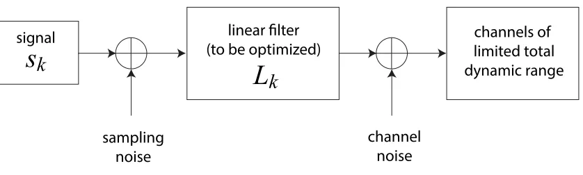
Figure 1: Schematic of optimization problem. Inthis problem we are constrained to encode signals 𝑠" in the presence of input and output noise with some linear filters,
denoted 𝐿".
As in Figure 1, assume 𝑠" are the variance of Gaussian signals (indexed by 𝑘) we
wish to encode using some type of linear filter, denoted 𝐿", in the presence of sampling
(input) noise, channel (output) noise, with a limited bandwidth. Without loss of
generality, we can take the sampling and channel noise to be unity, as we may rescale the
signal size for the former and the total dynamic range size for the latter. We expect the
sensitivity of the system to a particular signal to scale like the gain, |𝐿"|. We are still
constrained by the total output power of the system, 𝑃, and so the problem can be
formulated seeking to extremize the quantity 𝐼 = "𝐼"+ 𝛬𝑃. Here 𝐼 is the quantity to be
extremized with respect to 𝐿", 𝐼" is the mutual information between the channel input and
output, and 𝛬 is the Lagrange multiplier used here to enforce the power constraint.
Non-trivial solutions occur for 0 < 𝛬 < 1, and as 𝛬 moves from 0 to 1, the constraints switch
s
k
L
k
sampling noise
channel noise linear filter
(to be optimized) limited totalchannels of
14
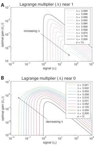
from being dominated by input-noise to being dominated by output-noise. This is worked
out in detail in [15] by setting 𝜕𝐼/𝜕𝐿" = 0 and 𝜕𝐼/𝜕𝛬 = 0. The solutions are given by
𝐿" 1 = − 2 + 𝑠"1 + 𝑠"4+ 4𝑠"1/𝛬
2(1 + 𝑠"1)
when the quantity is positive, and 0 otherwise. This quantity is positive as long as 𝑠" >
𝛬/(1 − 𝛬). This captures the intuition that sufficiently small signals are not worth
encoding. For 0 < 𝛬 < 1, when 𝛬 is near 1, the critical value of 𝑠" becomes infinite,
which corresponds to the transmission-limited, or output-noise limited regime. This
implies nothing but the largest of signals are worth encoding at all. When 𝛬 is near 0, this
critical value of 𝑠" approaches 0, which corresponds to the transmission limited, or
input-noise limited regime. In this situation, virtually all signals are worth encoding. Numeric
solutions depicting the resulting gain as a function of the signal strength are plotted in
Figure 2.
In the transmission-limited regime (𝛬 near 1), signals below the threshold value
have zero gain, and for large signal values, the asymptotic limit of the gain equation for
large signal strengths is given by
𝐿" 1~1/𝛬 − 1
15
Figure 2: Numeric depiction of different efficient coding regimes. Plots show the optimal gain, |𝐿"|, as a function of signal strength for varying levels of 𝛬, the Lagrange multiplier which enforces the output power constraint. Whenever 𝑠" < 𝛬/ (1 − 𝛬), the signal is
not encoded. Panel A depicts 𝛬 near 1, the transmission limited regime, where the gain of a signal is inversely proportional to the signal strength (|𝐿"|~1/𝑠"). Panel B depicts 𝛬
near 0, the sampling limited regime, where the gain of a signal is inversely proportional to the signal strength (|𝐿"|~ 𝑠").
10−2 10−1 100 101 102 103 10−3
10−2 10−1 100 101
Lagrange multiplier (
Λ
) near 0
Lagrange multiplier (
Λ
) near 1
Λ = 0.001
Λ = 0.002 Λ = 0.004
Λ = 0.008
Λ = 0.016
Λ = 0.031
Λ = 0.062 Λ = 0.125 Λ = 0.250 Λ = 0.500
a s
decreasingΛ increasingΛ
optimal gain (|
Lk
|)
A
B
Λ = 0.999
Λ = 0.998
Λ = 0.996
Λ = 0.992 Λ = 0.984
Λ = 0.969
Λ = 0.938
Λ = 0.875 Λ = 0.750 Λ = 0.500
a = 1/s
optimal gain (|
Lk
|)
signal (sk)
10−2 10−1 100 101 102 103 10
10−2 10−1 10 10
signal (sk)
16
This can be understood with the intuition that when signals are highly reliable, it is
optimal to spend an equal amount of bandwidth encoding each one. The gain here is
matched to compress the signal to fit into a fixed amount of bandwidth ( 𝐿" ~1/𝑠").
There is also a very sharp transition between the signals which are encoded according to
this bandwidth-equalizing intuition, and those which are not worth encoding at all. This is
depicted numerically in Figure 2A.
In the sampling-limited regime (𝛬 near 0), signals below the threshold value still
have zero gain, but there is a much larger transition region between the signals which are
not encoded and the reliable signals. The asymptotic form of the gain equation under the
conditions of 𝛬 near 0 is
𝐿" 1~ 𝑠"
1 + 𝑠"1 1 𝛬
If we examine the region 𝛬 < 𝑠" < 1, where the signal is smaller than the sampling
noise, but larger than the threshold for encoding, we see that the gain increases with the
signal size (𝐿"~𝑠":/1𝛬;:/4). This is plotted in Figure 2B. This regime quantifies the
intuition that, when signals are relatively unreliable, more resources should be spent on
those which are more reliable. For the purposes of analyzing signals which inherently
possess significant sampling limitations, this regime is likely to be more relevant.
Consider, for example, visual textures. The relevant properties have significant statistical
structure which needs to be averaged over some large homogeneous spatial region in
order to have a measurement with small error, but spatial variations are significant in
17
the important spatial variations, measurements of such statistics will be inherently noisy.
This motivates our hypothesis that human perceptual sensitivity to a visual texture
(quantified by a signal computed from images) should grow with the variability
(measured from natural visual scenes) of its signal.
Parameterizing a tractable set of visual textures
One of the powerful implications of the efficient coding hypothesis involves the
sensitivity of the population which encodes the relevant features of the natural world.
This sensitivity is something which any population, regardless of the particular encoding
scheme, should achieve. It is therefore possible, as long as we have a well-controlled
stimulus, to test the efficient coding hypothesis without knowing anything about the
actual underlying representation. By simply examining behavioral sensitivity to a
well-parameterized stimulus, and comparing the behavioral sensitivities to the presence of
these signals in natural images we can test predictions of the efficient coding hypothesis
at a macroscopic level. Our collaboration has previously tested this by looking at specific
patterns and classifying them as either informative (belonging to the coding region) or
uninformative (belonging to the zero gain region) based on whether or not they are
informative about natural scenes [14]. Our goal here is to probe these predictions in
greater depth by comparing the sensitivities to multiple patterns which are all predicted to
be encoded by the sensory system.
Generically, visual textures are motifs with a particular small-scale structure that
is repeated over a large region of the visual environment. The number of parameters one
18
the possible colorings of the regions. It is therefore most prudent to start with the simplest
tractable subset of these textures which can capture important two-dimensional spatial
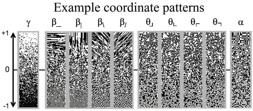
structure. We therefore constrain ourselves to considering 2x2 pixel motifs containing
only black and white pixels. There are 21×1= 16 possible configurations such a grid can
take, and a visual texture of this class can be described by the probabilities of each
coloring. Probability summing to 1 and translation invariance reduce the number of free
parameters to 10. A convenient basis to describe these is given by the general discrete
Fourier transform and contains one first-order coordinate (𝛾), four second-order
coordinates (𝛽;, 𝛽|, 𝛽/, 𝛽\), four third-order coordinates ( 𝜃∟ and rotations), and one
fourth-order coordinate (𝛼). For more details about this showing this is a complete
representation, see [16]. For any patch, computing these quantities is straightforward.
Each of these coordinates has a specific configuration of pixels, and the value it takes for
one example configuration is given by the parity of the pixels contained, taking black to
be -1 and white to be +1. The coordinate value describing an image patch is the average
across every matching configuration contained in the image patch. So −1 1
1 −1 has
𝛽; = −1, as there are two horizontal pixel configurations with the values 𝛽; −1 1 =
19
Figure 3: Visualizing 2x2 binary textures with single coordinates specified. Midline is white noise, and moving up or down in each column corresponds to increasing or decreasing the average value of the indicated coordinate. The emergent structures are
easily visible at the extreme ends of the spectrum.
Figure 4: Visualizing 2x2 binary textures with multiple coordinates specified.Center point is white noise, and moving outward the patterns generated use increasingly strong
coordinates. The emergent structures are easily visible at the extreme ends of the spectrum, and the combination of two coordinates provides significantly different patterns from only specifying one. There exist restricted regions (e.g. gray region of right
20
It is possible to generate image samples which are maximum entropy subject to the
constraint of having 1 or 2 coordinates specified [16] , and examples of the appearance of
these patterns appear in Figures 3 and 4. To provide some intuition for this algorithm,
consider the simple case of specifying single coordinates. It is easy to identify a boundary
which contains only uncoupled pixels, which may be generated randomly. From here, the
relevant template shape may be shifted in such a way that only one pixel is undefined.
The pixel color is chosen from the Boltzmann distribution, enforcing the constraint on the
average coordinate value for the image. For example, specifying the 𝛽; coordinate leaves
independent rows, and so in each row, we may randomly generate the left-most pixel. We
may sequentially generate pixel 𝑖 + 1 according to the distribution 𝑝 𝑐HI: =
:
J𝑒;LMLNO (PQ)RSRSTU. The functional form of this equation is identical to a formulation of
the one-dimensional Ising model that specifies the spin-spin correlation rather than the
coupling strength.
Characterizing the “natural” visual environment using visual textures
The efficient coding hypothesis claims that sensory systems of organisms haveevolved in order to be able to efficiently represent the types of stimuli they naturally
encounter. In order to remain faithful to this claim, we use images from the UPenn
Natural Image Database. The images are taken from natural baboon habitats in Botswana
using a camera calibrated to faithfully capture the responses that L, M, and S cones of
primates [17], although we cross-checked our work with another popular image
database(the van Hateren Image Database). Since we will be eventually making a
21
image as the most relevant element, though certainly more generic visual textures of
interest contain more generic color patterns. But what is the most sensible way to retain
the structure of a grayscale image after converting to a binary image? Natural images
have well-documented long-range correlations, which can be understood to a large extent
by the properties of translation-invariance and scale-invariance [18]. The former can be
understood by virtue of the fact that shifting a natural scene, for example to the left or to
the right, yields another natural scene. The intuition explaining the notion of
scale-invariance in natural images is as follows: if a particular environment or set of objects
constitutes one natural image, then so does the same set of objects as viewed from either
half the distance or twice the distance. These seemingly simple observations have
powerful implications about the statistical properties of natural images, including the
typical pair correlation between pixels. The fact that natural images have long-range
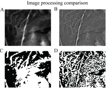
pixel-pixel correlations implies that simply binarizing the grayscale image by itself (e.g.
about the pixel intensity median) leaves large regions of the image either entirely black or
entirely white and removes much of the small-scale structure of the image. This is a
property which holds across the ensemble of images, and is itself unhelpful in
distinguishing individual images from one another. By only removing the average pair
correlation across the entire database (a procedure called whitening), we leave excess
correlations that exist in specific images, and therefore don’t lose any information that
can be used to distinguish images. The difference in these two methods is illustrated in
Figure 5. The whitening filter has a center-surround structure reminiscent of some retinal
ganglion cells, and we have discussed arguments that the purpose of some early visual
22
Figure 5: Comparing binarized images with and without removing average pair correlation. In panel A, the original image of a baboon’s face slightly obscured by some
brush. In panel B, the image has been filtered in order to remove the average pair correlation from the dataset. The significant features of the image are still visible. In
panel C, the original image (panel A) has been binarized by setting all pixels with luminance higher than the median to 1, and all other to zero. Information about many local features, such as fur texture, are completely absent due to the strength of long-range
correlations. In panel D, the whitened image (panel B) has been binarized about its median pixel intensity. Much more local information, such as the grass’s countour and
23
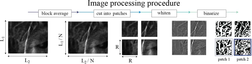
In order to check that scale does not affect the results, we introduce the
block-average factor 𝑁 which sets the scale of the image by shrinking the image by a factor of
𝑁 in each direction, whose pixel values are the average of the corresponding 𝑁×𝑁 block
in the original image. We do not assume scale invariance holds in the natural images, so
we will remove the average pair correlation computed empirically from the natural image
dataset used. This is done by flattening the average Fourier power spectrum, which relies
on translation invariance.1 To reliably estimate the pair-correlation for an image with 𝑃
pixels, we need approximately 𝑃1 images (or 𝑃 images if we assume
translation-invariance). Since our nice-sized databases have ~1000 images with ~1 Megapixels each,
it is obvious that we will not have enough data to compute these quantities for full-sized
images. Instead, we cut the original images into image patches of size 𝑅×𝑅 to form a
larger database of smaller images. With these choices in image processing parameters, we
can additionally test the results to see whether or not the scale of the image analyses has
any bearing on the texture representations. The full processing procedure is pictured in
Figure 6.
1Another way to achieve this result is by computing the principle components of the
24
Figure 6: Depiction of image processing procedure. We first take an ensemble of images and make new pixels by averaging blocks of 𝑁×𝑁 pixels to make effective pixels in order to test the analysis across scales. We then divide the new image into patches of size
𝑅×𝑅 in order to be able to have enough samples to make meaningful ensemble statistics. This provides another check on scale invariance for the estimation of statistics. The
image patches are then whitened in order to remove the mean pair-correlation. The whitened image is binarized at its pixel-intensity median, yielding a binary image which contains much of the structure at all length scales. The binarized image patches are used
to compute the distribution of texture parameter values across natural images.
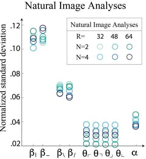
Once we have these image patches, we may compute the distributions of the
various texture parameter values (in the manner described above) in order to see which
are the most informative ones about natural scenes, and therefore, the ones to which we
expect people to be most sensitive. We compute the mean of each of the texture
parameters in each image patch, and our distribution contains one such vector for each
image patch in the analysis. The standard deviation of this distribution, which we
consider here to represent the strength of the signal from the above efficient coding
calculation, is plotted for single coordinates in Figure 7. A single scale factor for the
overall vector length was used for each set of image processing parameters. This can
account for overall variance differences that can arise due to larger image patches having
inherently smaller variances. Interestingly, non-trivial structure has already begun to
25
Figure 7: Normalized standard deviation of single coordinates. Here, we see the horizontal and vertical two-point correlations are most prominent, followed by diagonal
two-point correlations. Four-point correlations are more prominent than three-point correlations of any orientation. Despite the apparent overlap in the cloud of points, rank
ordering is preserved for each individual analysis.
strongest, followed by diagonal two-point correlations. Three-point correlations are the
least prominent, with smaller variance than the four-point correlation. Performing this
analysis on white noise yields equal standard deviation in each coordinate direction,
suggesting that these are indeed novel features characterizing natural images.
Characterizing human sensitivity to visual textures
To draw an analogy to the efficient coding hypothesis above, we interpret the
ideal amount of gain to apply to a signal to be proportional to the sensitivity a subject
displays to the signal. This means that we do not need to measure from the entire neural
26
signals, but rather we know the effective gain applied by measuring the psychophysical
sensitivity. Additionally, it is worth noting that neural representations supporting
discrimination of this kind of visual texture do not emerge until, at the earliest, secondary
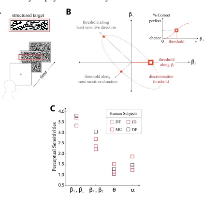
visual cortex (V2) [19]. In order to test human sensitivity to these visual textures, we use
a four-alternative forced-choice task (see Figure 8A), in which a strip with a specific set
of parameter values is placed in one of four locations (top, bottom, left, or right) and the
rest of the image is filled with white noise. More specifically, the subject is asked to
fixate at a point on a screen, after which the image changes to the structured target on
white noise background for 120ms, before a white noise washout image is displayed to
prevent the user from utilizing the afterimage. The task reflects the ability of the subject
to distinguish the texture from white noise. This is done for a variety of coordinate values
(specifying single and dual coordinate values), from which a threshold is defined as the
strength of a parameter required for a subject to distinguish the location of the texture
with an accuracy of 62.5% (halfway between chance and perfect) as schematized in
Figure 8, panel B. An early observation about the psychophysical sensitivities shows that
human subjects are symmetrically sensitive to positive correlations as negative
correlations. There is no reason that this needs to be the case, although it is a property
that an ideal observer would exhibit. The results from single-coordinate measurements
feature the same rank-ordering as in the natural image analyses, β;, β| > β/, β\ > α > θ.
Here, due to the indistinguishability of thresholds for some classes of texture parameters,
27
Figure 8: Depiction of psychophysical experimental procedure. The task (schematized in A) requires the subject to fixate on the center of the screen before the structured image is displayed. After 120ms, a white noise image is displayed to prevent burn in. The subject has to identify the location of the structured part of the image (top/bottom/left/right). This
is done for a variety of texture parameter values, allowing the calculation of a threshold (where the subject reaches halfway between chance and perfect) for each coordinate, as
well as oblique directions in each 2-dimensional subplane(panel B). The results for single-coordinates are displayed in panel C, featuring the same rank-ordering as found in
28
class, as seen in Figure 8, panel C. This is very different from what an ideal observer
would display, which would be equal sensitivity in each single coordinate direction [16].
Each subject performed 4320 trials per plane, totaling 47520. For more details about the
psychophysical experimental procedures, see [20].
Comparing natural image statistics to human psychophysical sensitivities
Since we expect the sensitivity to grow with the signal strength, and thepsychophysical threshold to be small for parameters to which we are very sensitive, we
should compare the standard deviations found in natural images to the inverse of the
psychophysical threshold. After allowing for a single overall scale factor for each set of
image processing parameters, plotting these quantities against one another (see Figure
9A) shows a striking degree of similarity. In addition to the robustly preserved
rank-ordering, the relative magnitudes of the standard deviations match the relative
magnitudes of the psychophysical sensitivities. It is also interesting to observe that the
variability between image analysis parameters is similar to the variability between
subjects.
Seeing this striking level of agreement for individual coordinates is very
interesting, but our choice of single coordinates was simply using a convenient basis,
rather than describing a fundamental set of independent parameters. We therefore need to
examine the covariance structure of these signals, and compare the thresholds predicted
by the inverse covariance matrix given from the natural image statistics to the threshold
ellipses measured from human subjects. A comparison of these ellipses is shown in
29
Figure 9: Comparing natural image statistics to psychophysical sensitivities. In panel A, the psychophysical sensitivity, given by 1/threshold, is plotted in red. Natural image standard deviations, plotted in green-blue, have each been allowed a single scale factor
for each set of processing parameters, since the overall magnitudes need not directly reflect the psychophysical sensitivity. The degree of variability in image analyses is similar to the degree of variability between subjects. In panel B, the threshold ellipses for
30
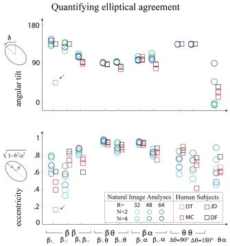
although results are similar across image analyses as well (for more detailed
measurement, see [2]). We quantified the elliptical parameters, eccentricity and tilt, to
measure the agreement (see Figure 10) between the ellipses, but note that when
eccentricity is small, tilt becomes meaningless. Note that for the elliptical parameters,
there is no scale factor at all, and the prediction made here has no free parameters, as the
scale factor only affects the overall size of the ellipse.
Figure 10: Quantifying elliptical agreement. Angular tilt (top) and eccentricity (bottom) plotted for a variety of image processing parameters and each human subject. The eccentricities and tilts agree to a large extent. This comparison is parameter free, as the
31
Discussion of binary results
Here, we have proposed an idea governing the organization of neural circuits that
makes predictions at the level of human behavior. This is a very powerful statement
about the nature of neural circuit organization. For the purposes of this study, we did not
even need to make direct measurements of cortical activity. The intuition behind the
suggested coding scheme is that for signals which have relatively high uncertainty, it is
worth devoting more resources to looking at signals that are more variable. In this case,
sampling limitations for local texture features imply that signals with larger variability
are more useful in distinguishing between natural images. It is interesting to note that a
strength of the comparison made here is between a set of artificial textures and statistics
computed from natural scenes. A strength of this study is that, despite the seemingly
unnatural structure of the artificial stimuli, we were able to predict their salience to
human subjects based on observations about how the texture parameters characterize
natural images.
It is also interesting to note that the perceptual thresholds likely arise from cortical
processing, as this implies that the efficient coding hypothesis is not only a useful tool to
apply in the extreme sensory periphery, but can useful for understanding central
processing as well. The stimuli contrast was very high, and the pixels were easily visible
(14 arcmin), meaning that retinal limitations for contrast sensitivity and spatial resolution
were not limiting factors for the discrimination. It has also been shown that cat retinal
populations show no sensitivity to the four-point correlations, but simultaneous visual
cortex field potential measurements do [21]. Similarly, neurons in macaque visual cortex
32
coding regime that makes these predictions has input-noise as the dominating parameter
limiting performance, which differs from the one traditionally applied to understand
peripheral vision. In peripheral vision, the optic nerve applies a heavy constraint to output
power, and output noise is the limiting factor. The ‘whitening’ regime, as it is called,
calls for neural resources to be devoted with an inverse relation to the variability. For
example, the retina has greater sensitivity for low spatial frequencies than high spatial
frequencies, reflecting the ~1/𝑓1 power spectrum observed in natural images. This
difference in coding constraints observed for peripheral and cortical vision could provide
important insights into coding strategies used elsewhere in cortex.
It is also interesting to note that we observed more evidence for scale invariance
in natural images. Image analysis parameters changing the scale of the scene (block
average factor) did not significantly alter any of the significant findings of these texture
statistics, which suggests scale invariance is a useful way of thinking about natural scenes
in more ways than just predicting the frequently observed 1/𝑓1 power spectrum.
This work is building on a larger class of studies examining the role of neural
coding for visual texture perception. Previous studies within our own collaboration [14]
have shown that certain high-order correlations that are present in natural scenes are not
perceptually salient at all, finding that their presence in natural scenes is entirely
explainable from shorter-range correlations. Other studies [22], have found manipulations
to higher-order statistics in images that deform images in a manner that are undetectable
to a fixating human(but readily observed when your gaze wanders). Both of these studies
33
elements which fit into the non-coding region. We have taken this a step further and
shown that, for higher-order correlations that humans are sensitive to, we seem to be
sensitive to them in proportion to their variability.
Another interesting implication of this line of work applies to situations that rely
on human experts to examine highly unnatural images. In medical imaging, for example,
it can be very difficult for an untrained eye to spot a defect or a fracture, particularly in a
small bone or the appearance of a small tumor. It may be possible that these types of
images, which certainly have highly different statistics from natural images, have a
significant amount of information stored in local correlations that are difficult for humans
to detect. If it were possible to effectively ‘rotate’ the coordinates so that the informative
ones align with the ones humans are naturally sensitive to, it may make diagnoses based
on medical image data much easier and more reliable. Some research in this direction has
already begun.
Extension to grayscale images
It is of course natural to want to extend these kinds analyses to grayscale images,
as our experience of the world has nearly a continuum of luminance values, rather than
just black and white. Analogous grayscale textures can be computed using the methods
established in [16]for finite grayscale levels. We will start by examining textures with 3
grayscale levels in the same 2x2 pixel block. The basis we will use is related to the
number theoretic Fourier transform, and spending some time describing this will be
useful. In a 2x2 grid, we can label the pixels starting at the top left and going clockwise
34
letters, so 𝐴𝐵 will denote a horizontal 2-point correlation, while 𝐵𝐶𝐷 denotes a 3-point
correlation in a configuration that excludes the top-left corner. Previously, with only two
grayscale levels, we used the parity of the block. Now, it is helpful to think of the patterns
with respect to arithmetic mod 3, where a black pixel is labelled 0, a gray pixel labelled 1,
and a white pixel labelled 2. Since each of these individual patterns is well-defined, we
can deconstruct it into probabilities that the sum of individual grayscale values is equal to
a specific value. For example, the 𝐴𝐵:1 coordinate has probabilities associated with
𝑃(𝐴 + 2𝐵 = 0 𝑚𝑜𝑑 3), 𝑃(𝐴 + 2𝐵 = 1 𝑚𝑜𝑑 3), and 𝑃(𝐴 + 2𝐵 = 2 𝑚𝑜𝑑 3). These
probabilities must sum to 1, and so there are only two free parameters describing this
coordinate subspace. In the binary case, we had only a single value to describe these
coordinates because there were two possible values the combined coloring could take.
The patterns generated by this 𝐴𝐵:1 are that 𝐴 = 𝐵, so no change as pixels move in the
horizontal direction [000…/111…/222… depending on initial value] when
𝑃 𝐴 + 2𝐵 = 0 𝑚𝑜𝑑 3 = 1; the cyclic pattern [0210210…] when 𝑃 𝐴 + 2𝐵 =
1 𝑚𝑜𝑑 3 = 1; and the cyclic pattern [012012…] when 𝑃 𝐴 + 2𝐵 = 2 𝑚𝑜𝑑 3 = 1. The
subspace of values these three probabilities can take lies within a triangle bounded by the
three probabilities taking values between 0 and 1, and summing to 1. Overall, there are 33
different patterns, each with two degrees of freedom, totaling 66 dimensions (2
first-order, 16 second-first-order, 32 third-first-order, 16 fourth-order).
We can compute these quantities for natural images following a very similar
processing pipeline as before, but instead of binarizing at the pixel intensity median, we
35
distributions of these parameters in natural images. Psychophysical measurements have
been carried out to analyze human sensitivity to several subspaces [23]. We will compare
some our analyses of these natural scene statistics to the psychophysical measurements.
Comparing the thresholds predicted using the same analyses to a subset of the planes
containing 2-point correlations (plotted in Figure 11), we see agreement in the orientation
and eccentricity of the ellipses for two subplanes (𝐴𝐵:1 and 𝐴𝐷:1), but a lack of such
strong agreement in two other less eccentric planes (𝐴𝐵:: and 𝐴𝐷::). This is an
interesting finding in its own right, and remains to be seen why agreement exists in some
ways, but not in others. One possibility is that the neural mechanisms for encoding these
highly complex features are heuristic, and therefore unable to capture every detail of the
distribution, but prioritize coding the most important and salient features.
To further analyze this data, it is useful to use principle component analysis
(PCA) to analyze where the bulk of the distribution is concentrated. Upon doing so, the
first interesting feature that pops up is the eigenvalue spectrum (plotted in Figure 12A).
There are 99 principle components because the covariance analysis here is performed
using the full probability values, but 35 dimensions are null. This is expected because
normalization reduces the number of free parameters to 66, and our “trinarization”
process fixes the probability of having each, black, white and gray colored pixels. Then,
we observe that the bulk of the eigenvalues are quite small compared to the variance of
the first few components. In fact, nearly 75% of the variance in the dataset is contained
within the first 10 principle components. These first 10 principle components are
36
fourth-order statistics. This is consistent with the psychophysical observation that many
second-order statistics are salient, but few third- and fourth-order ones are. Furthermore,
the principle components provide insight into the natural structure of visual scenes, and
may provide insight into the kinds of symmetries we may expect to observe
psychophysically. As an example, plotted in Figure 12B, are coefficients of three of the
first five principle components. The first column corresponds to the probability that the
sum is equal to zero, the second column to the sum being one, the third to the sum being
two. The principle component that contains the largest amount of variance in the data
contains has the most significant contributions occurring equally from 𝐴𝐵:1, 𝐴𝐶:1, 𝐵𝐶:1,
and 𝐴𝐷:1 (and the relevant sum equaling zero), all with positive coefficients. An
interesting feature of this vector is that it is approximately symmetric under rotating the
underlying image by 𝜋/4. Two more of the first few principle components contain
similar contributions from two-point correlations that span a similar subspace as the most
significant component, but differ in that positive and negative coefficients imply that this
element is actually antisymmetric under the operation of rotating the image by 𝜋/4. This
natural symmetry may manifest itself in an important way, and suggests that one
non-trivial two-dimensional subspace of interest is, for example, the 𝑃 𝐴𝐵:1= 0 −
𝑃(𝐴𝐶:1= 0) plane, because we have strong predictors along oblique directions within
this plane. This analysis would additionally shed light on the role of this underlying