FLOW ROUTING THROUGH A TANK CASCADE SYSTEM IN A SEMI ARID CATCHMENT USING A PHYSICALLY BASED MODEL

165 | P a g e

FLOW ROUTING THROUGH A TANK CASCADE

SYSTEM IN A SEMI ARID CATCHMENT USING A

PHYSICALLY BASED MODEL

N.C.Arun

1

Assistant Professor, Civil Engineering Department,

Kongunadu college of Engineering and Technology, Trichy, Tamil Nadu, India

ABSTRACT

Among the most basic challenges of hydrology are the quantitative understanding of the processes of runoff generation and prediction of the flow hydrographs and their transmission to the outlet. Traditional techniques have been widely applied for the estimation of runoff hydrographs at the outlets of gauged watersheds using historical rainfall-runoff data and unit hydrographs derived from them. Such procedures are questioned for their reliability due to the climatic and physical changes in the watershed and their application to semiarid catchments and hence modelling of the area becomes necessary.Hydrology constitutes a fundamental study component, known as Rainfall Runoff Modelling. These models are applied universally for various catchments, micro to macro levels. Reliable estimates of stream flow generated from catchments are required as part of the information sets that help policy makers make informed decisions on water planning and management. The characteristics of the streamflow time series that influence water resources system modelling and planning can include the sequencing of flows on daily and longer time steps, spatial and temporal variability of flows, seasonal distribution and characteristics of high and low flows.An approach to hydrological modelling is to seek to develop "physics-based models," i.e. models explicitly based on the best available understanding of the physics of hydrological processes. Such models are based on a continuum representation of catchment processes and the equations of motion of the constituent processes are solved numerically using a grid, of course discretized relatively crudely in catchment-scale applications. In the present thesis a modified version of the physically-based distributed MIKE SHE model code has been applied to the Sindapalli Uppodai sub-basin using conventional and remotely sensed data .The Fifteen tanks forming a tank cascade system in Sindapalli Uppodai sub-basin are considered for the present study. The flow routing on the ground surface is calculated by MIKESHE’s Overland Flow Module, using the diffusive wave approximation of the Saint Venant equation. The hydrograph of routed runoff from the tank cascaded catchment using physically based model is developed.

Key words:

;

;

;

;

1. INTRODUCTION

Water is one of nature's most important gifts to mankind. Essential to life, a person's survival depends on

drinking water. In the hydrological cycle; water evaporates from the oceans, lakes and rivers, from the soil and

166 | P a g e snow. It infiltrates to the groundwater and discharges to streams and rivers as baseflow. It also runs off directly

to streams and rivers that flow back to the ocean.

2. PAST RESEARCH

Bahaa-eldin E. A. Rahim et al. (2005) used the fully distributed physically based MIKE SHE modelling system

was used to simulate the individual hydrological components of the total water balance for the Paya Indah

Wetlands (PIW) watershed in the west of Peninsular Malaysia. Results reveal that the overall water balance is

predominantly controlled by climate variables. Estimation of total water balance is a substantial issue for

watershed modelling in order to simulate the major components of the hydrological cycle to determine the stress

of different anthropogenic activities on the available water resources within a catchment.. Application of the

model to the PIW watershed provides detailed estimation of the total water balance for a first-order catchment in

which actual evapotranspiration (ET) represents approximately 65 and 58%, while overland flow (OL) to the

PIW lake system represents 12.38 and 12.3% of the total rainfall during the calibration and validation periods,

respectively. The difference of the inflow and outflow was taken as storage in depth. Overall, the model gives a

reasonable output of total error of less than 1% of the total rainfall, which in turn indicates that the interaction

among components is satisfactorily sustained.

The MIKE SHE model is a fully integrated watershed model that simulates all the major processes occurring in

the land phase of the hydrologic cycle. Developed by three European organizations (Danish Hydraulic Institute,

British Institute of Hydrology and the French consulting company SOGREAH) and sponsored by the

Commission of the European Communities, it was originally named SHE (Système Hydrologique Européen)

model. This deterministic, fully distributed, and physically-based model is used mostly at the watershed scale

and from a single soil profile to several sub-watersheds with different soil types. The model's distributed nature

allows a spatial distribution of watershed parameters, climate variables, and hydrological response through an

orthogonal grid network and column of horizontal layers at each grid square in the horizontal and vertical,

respectively. Being physically-based, the topography along with watershed characteristics (vegetation and soil

properties) is included into the model. The MIKE SHE model has a modular structure, enabling data exchange

between components as well as addition of new components. The flexible operating structure of MIKE SHE

allows the use of as many or as few components of the model, based on availability of data. (Abbott et al.,

1986a).

3. STUDY AREA AND DATABASE

3.1. LOCATION

Vaippar basin located in the southern part of Tamilnadu, India was chosen as study area. The basin lies between

North Latitude of 8° 59‟ and 9° 49‟ and East longitude of 77º15‟ and 78º23‟ covering total area of 5423 km². An

index map of Vaippar basin is presented in the figure 3.1. There are two major river systems present in Vaippar

167 | P a g e draining the basin. The basin is bounded by Vagai basin and Western Ghats, Gulf of Mannar, Thamiraparani

and Kallar River basins and Gundar River basin.

3.2 HYDROMETEOROLOCAL CHARACTERISTICS

3.2.1 Climate

The climate of the region is semi-arid tropical monsoon type. It has a high mean temperature and a low

degree of humidity. The temperatures range from 20º C to 37º C. April, May and June are the hottest months of

the year.

3.2.2 Rainfall

The Vaippar basin lies a low rainfall belt having an annual average rainfall of 772 mm. Southwest monsoons

contributes 148 mm (20%), while Northeast monsoon contribution 414 mm (53%). The basin receives a major

share of its annual rainfall during Northeast monsoon. This monsoon helps to build up storage in the reservoirs

and tanks both system and non-system. This basin has Western Ghats on Western side. Southwest monsoon

rainfall, though lesser that the North East monsoon rainfall, still contributes some run off helping to build up

storage in Pilavukkal reservoir.

3.3 SINDAPALLI UPPODAI SUB BASIN

Sindapalli Uppodai sub basin is a tributary of Nichanbanadhi and it originates in Sathur taluk and runs through

Sivakasi and Sathur taluk. The basin area is 177 km² and there Sivakasi rainfall stations have got more influence

than the Sathur rainfall station. The mean areal annual rainfall of the sub basin works out of 746 mm.

3.4 DRAINAGE PATTERN

Distinctive patterns are acquired by stream networks in consequence of adjustment to geologic structure. In the

early history of a network, and also when erosion is reactivated by earth movement or a fall in sea level, down

cutting by trunk streams and extension of tributaries are most rapid on weak rocks, especially if these are

impermeable, and along master joints and fault. The map showing the sixteen tanks in the Sindapalli Uppodai is

168 | P a g e Fig 3.2 Drainage Map of Sindapalli Uppodai sub basin

3.5 LAND USE

Land use map depicts the pattern of land use in the study area and is an important input for preparation of the

other theme maps. The land use describes what use a parcel of land is put to, e.g. residential, industrial,

commercial, agricultural etc. It has also been defined as "the arrangements, activities and inputs people

undertake in a certain land cover type to produce, change or maintain it. The land use map of Sindapalli

Uppodai is presented.

3.6 DATA COLLECTION

Data collection is done as the one important phase in the thesis work. The data collected would ensure

the result obtained out of the particular study. As a part of thesis work, the toposheet 58 G 11 & 15 is collected

from the Survey of India and is digitized and then the particular study area the Sindapalli Uppodai is delineated

using the Arc GIS 9.3.

4

METHODOLOGY

4.1 GENERAL

The flow over the land was simulated using diffusive wave approximation of St.Venant‟s equation. For

two-dimensional surface water flow, it is common to simplify the governing equations by neglecting momentum

losses due to lateral inflows, and local and convective accelerations. This is known as the diffusive wave

approximation, which is implemented in MIKESHE using 2D, finite-difference approach.

4.2 FINITE DIFFERENCE METHOD

The finite difference approximations for derivatives are one of the simplest and of the oldest methods to solve

differential equations. In mathematics, finite-difference methods are numerical methods for approximating the

solutions to differential equations using finite difference equations to approximate derivatives. The principle of

Finite Difference Method is that the derivatives in the partial differential equation are approximated by linear

combinations of function values at the grid points. Briefly, the finite difference method can be characterized as

follows. Utilizes uniformly spaced grids. At each node, each derivative is approximated by an algebraic

expression which references the adjacent nodes. A system of algebraic equations is obtained by evaluating the

169 | P a g e

4.3 Methodology of flow routing using diffusive wave approximation

4.4.MODEL INPUTS:

4.4.1 Model domain and grid:

Regardless of the components included in the model, the first step in the model development is to

define the model area. On a catchment scale, the model boundary is typically a topographic divide. The map is

loaded as a shape file and the catchment shape is displayed in the overview box. The screenshot of the model

domain.

4.4.2 Manning’s M:

Another watershed characteristic required by the model is surface roughness coefficient or Manning„s M, the reciprocal of Manning„s n, for the different land uses. The values of Manning„s n were taken from Venti Chow.

170 | P a g e

4.4.3 Detention Storage:

Detention Storage is used to limit the amount of water that can flow over the ground surface. The depth

of ponded water must exceed the detention storage before water will flow as sheet flow to the adjacent cell.

Taken as 0.2mm

4.4.4 Initial water depth:

The measured surface water depth was used to initialize the water depth above the ground surface for

the model to run. This is the initial condition for the overland flow calculations. The initial water depth is

usually zero. The initial water depth for overland flow is also the boundary condition for overland flow.

4.4.5 Precipitation rate:

The precipitation rate is the measured rainfall. The Precipitation Rate item comprises both a distribution

and a value. The distribution can be uniform, station-based or fully distributed. If the data is station-based then

for each station a sub-item will appear where one can enter the time series of values for the station. Precipitation

rates were specified as rainfall time series from three various rainfall stations namely Sattur, Sivakasi and

Vembakottai (as shown in the Figure 4.8) around the region .The coverage areas delineated by Thiessen

polygons

5.RESULTS

Overland flow is simulated for the period of 6 months (from May 2006 to December 2006) using

MIKESHE software. The results are presented in the from different visualization in terms of graphs, pictures,

animations.

5.1RESULTS OF SIMULATION:

All the simulation results are collected in the Results tab. This includes detailed time series output for

171 | P a g e

Fig 5.1 Screenshot of the results tab

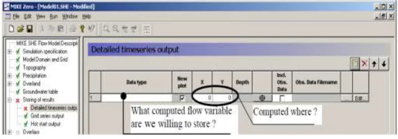
5.1.1 MIKESHE Detailed time series output:

Detailed time series output submenu allows the users to store the computed flow variables at each time step at

specific points. Click the dotted rectangle with a yellow spark in order to add a storage point as shown in the

Figure 5.2. A new line appears in the window. For each specified point, the output variable is stored in a .dfs0

file with one value for every simulation time step.

Fig 5.2 Detailed time series output

Finally, for each item in the detailed time series table, an HTML plot is created in the Result Tab.

The MIKE SHE detailed time series tab includes an HTML plot of each point selected in the detailed time series

output dialogue. Go and click the field „Data type‟: one are given choice between the variables that can be

stored as show in the figure 5.3

Fig 5.3 Screenshot of the Data Type

The detailed time series of the precipitation rate, depth of the overland water, overland flow in the x

direction and overland flow in the y direction are obtained for the simulation period at the specified outlet (as

172 | P a g e measurement stations. That is, locations at which a time series of measurements are available, for example,

water levels in a well or water depths on a flood plain. Overland flow in x-direction (this is the flow across the

boundary from celli to celli+1 in volume/time e.g. m3/s).

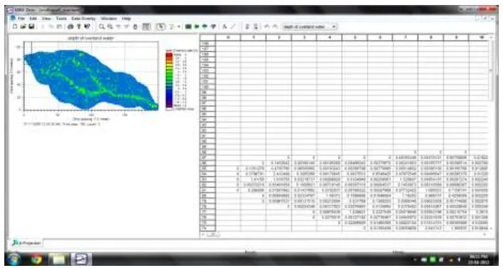
5.1.2 Gridded Data Result Viewer:

Go to „Gridded Data Result viewer‟ in order to visualise the results stored in the form of maps. The computed

variables stored in the result files are displayed in the right hand side window. The simulation results are stored

in a time-varying map file (extension .dfs2). There is one file for each simulation variable. The name and

location of the files are specified in the rightmost column of the right-hand side window. The (+) and (-)

magnifying glass icons are used to zoom in and out respectively. The blue clock-shaped icons allows us to go

forward or backward in time when the map is a time-varying one. If we click on a point of the map in the

left-hand side window, the numerical values around this point will be displayed in the right-left-hand side window that

looks like an Excel calculation sheet

Moreover, the shape of the region covered by the right-hand side window will be displayed on the map

of the left-hand side. The numerical values and the colour map are updated automatically as we go forward or

backward in time using the clock-shaped icons. The Gridded Data of Precipitation rate, Depth of overland

water, Overland flow in x direction, and Overland flow in y direction are show in the Fig.5.7, 5.8, 5.9 and fig

5.10 respectively. The output can also be obtained as .REV, an animation format which shows Precipitation rate,

Depth of overland water, Overland flow in x direction, and Overland flow in y direction as time frame for the

173 | P a g e AVI format). Various time frames of, depth of overland water, Overland flow in x direction, and Overland flow

in y direction are shown in the Fig 5.11, Fig 5.12 and 5.13 respectively.

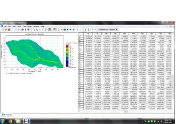
The result showed that the Depth of overland water, Overland flow in x direction, and Overland flow in y

direction are found to be higher in the month of November during the north east monsoon. The model simulated

the depth of overland water from „0‟ to 4 meters to the maximum near the tank and low elevation regions.

Overland flow in x direction is found to be from 0 to 4.5 m3/sec. Overland flow in y direction is found to be

from 0 to -16 m3/sec.

The flow rates in the x and y direction are calculated based on the sign of friction slopes in the x and y direction

respectively. The negative discharge implies that the flow direction is actually from (j.k) to (j,k-1) drainage

cells.

Fig 5.5 Overland computational time series output

174 | P a g e

Fig 5.9 Gridded Data of Overland flow in x direction ( m3/sec) on 11/07/2006

Fig 5.10 Gridded Data of Overland flow in y direction ( m3/sec) on 11/07/2006

A physically based, distributed overland flow routing model is developed to model runoff for a period of 6

months (May 2006 to December 2006) on Sindapalli Uppodai, a semi arid catchment. After reviewing various

Rainfall Runoff models and sufficiency of data from the study area, the MIKESHE model is selected. The flow

175 | P a g e module using 2D, finite-difference approach. The result showed that the Depth of overland water, Overland

flow in x direction, and Overland flow in y direction are found to be higher in the month of November during

the north east monsoon. The model simulated the depth of overland water from 0 to 4 meters to the maximum

near the tank and low elevation regions. Overland flow in x direction is found to be from 0 to 4.5 m3/sec.

Overland flow in y direction is found to be from 0 to -16 m3/sec. While the results may be considered

preliminary, the model shows potential for use with future refinements in input data.

 Results from the physically based model MIKESHE insights into both the strengths and weaknesses of the

combined model structure, parameters and input data as a tool for predicting runoff behaviour in the

Sindapalli Uppodai catchment.

 MIKE SHE system, a more general process-based framework allows us to select between a number of

different process descriptions and model structures.

 The MIKESHE modeling system is a complex modeling system, developed with the water movement

module as a foundation. It is capable of performing a variety of functions housed in its modular structure.

 MIKESHE has been found to be a very effective tool to handle large amount of both spatial and temporal

data, which are stored and retrieved for the estimation of runoff.

 The precision of model simulation depends upon DEM accuracy.

 The model needs more detailed calibration with field tests to derive any discerning results of quantitative

results and it should be validated.

REFERENCES

1. Abbott, M.B., J.C. Bathurst, J.A Cunge, P.E. O'Connell, and J. Rasmussen. (1986). “An introduction to the

European Hydrological System - Système Hydrologique Européen, "SHE", 1: History and philosophy of a

physically-based, distributed modelling system.” Journal of Hydrology. Vol.No.87, pp 45-59.

2. Bahaa-eldin E. A. Rahim1, Ismail Yusoff, Azmi M. Jafri, Zainudin Othman & Azman Abdul Ghani (2010),

“Application of MIKE SHE modelling system to set up a detailed water balance computation”, Journal of water and environment,Vol.3,pp55-63.

3. Brooks, K.N., P.F. Ffolliott, H.M. Gregersen, and J.L. Thames. (1991), a book on “Hydrology and the

Management of Watersheds”. pp 210-223.

4. Chulgyum Kim, Hyeonjun Kim, Sangjun Im (2008) “Assessing the impacts of land use changes on

watershed hydrology”. Journal of Environmental Geology,pp 231-239.

5. D. H. A. Al-Khudhairy (1999), “Hydrological modelling of a drained grazing marsh under agricultural land

use mulation of restoration anagement scenarios”, journal of hydrological sciences, Vol.6,pp 44-45.

6. Dingman, S.L.( 2002),a book on “ Physical Hydrology”. 2nd edition, pp 45-68.

7. Douglas Graham (2005), a book on “Flexible, integrated watershed modelling with MIKE SHE”, pp

245-272.

8. Li, Manliang Zhang, Shengping Wang, Zhiqiang Zhang (2008) “Evaluation of the mike she model for

176 | P a g e 9. Rajeev Raina (2004), a MS thesis on “Development of a cell-based streamflow routing model”, Graduate

studies of Texas A and M University.

10. Sakthivadivel R, (2003) “A simple water balance modelling approach for determining water availability in

an irrigation tank cascade system”. Journal of Hydrology Vol. 273, pp 81–102.

11. Shalini Oogathoo (2006), a MS thesis on “Runoff simulation in the Canagagigue creek watershed using the