University of Pennsylvania
ScholarlyCommons
Publicly Accessible Penn Dissertations
2017
Leveraging Privacy In Data Analysis
Ryan Michael Rogers
University of Pennsylvania, [email protected]
Follow this and additional works at:
https://repository.upenn.edu/edissertations
Part of the
Computer Sciences Commons
, and the
Statistics and Probability Commons
This paper is posted at ScholarlyCommons.https://repository.upenn.edu/edissertations/2554
For more information, please [email protected].
Recommended Citation
Leveraging Privacy In Data Analysis
Abstract
Data analysis is inherently adaptive, where previous results may influence which tests are carried out on a single dataset as part of a series of exploratory analyses. Unfortunately, classical statistical tools break down once the choice of analysis may depend on the dataset, which leads to overfitting and spurious conclusions. In this dissertation we put constraints on what type of analyses can be used adaptively on the same dataset in order to ensure valid conclusions are made. Following a line of work initiated from Dwork et al. [2015], we focus on extending the connection between differential privacy and adaptive data analysis.
Our first contribution follows work presented in Rogers et al. [2016]. We generalize and unify previous works in the area by showing that the generalization properties of (approximately) differentially private algorithms can be used to give valid p-value corrections in adaptive hypothesis testing while recovering results for statistical and low-sensitivity queries. One of the main benefits of differential privacy is that it composes, i.e. the combination of several differentially private algorithms is itself differentially private and the privacy parameters degrade sublinearly. However, we can only apply the composition theorems when the privacy parameters are all fixed up front. Our second contribution then presents a framework for obtaining
composition theorems when the privacy parameters, along with the number of procedures that are to be used, need not be fixed up front and can be adjusted adaptively Rogers et al. [2016]. These contributions are only useful if there actually exists some differentially private procedures that a data analyst would want to use. Hence, we present differentially private hypothesis tests for categorical data based on the classical chi-square hypothesis tests (Gaboardi et al. [2016], Kifer Rogers [2017]).
Degree Type Dissertation
Degree Name
Doctor of Philosophy (PhD)
Graduate Group Applied Mathematics
First Advisor Michael Kearns
Second Advisor Aaron Roth
Keywords
Adaptive Data Analysis, Differential Privacy, Statistics
Subject Categories
LEVERAGING PRIVACY IN DATA ANALYSIS
Ryan Michael Rogers
A DISSERTATION
in
Applied Mathematics and Computational Science
Presented to the Faculties of the University of Pennsylvania in Partial Fulfillment of the Requirements for the Degree of Doctor of Philosophy
2017
Supervisor of Dissertation
Michael Kearns, Professor of Computer and Information Science and National Center Chair
Co-Supervisor of Dissertation
Aaron Roth, Associate Professor of Computer and Information Science
Graduate Group Chairperson
Charles L. Epstein, Thomas A. Scott Professor of Mathematics
Dissertation Committee
LEVERAGING PRIVACY IN DATA ANALYSIS
c
COPYRIGHT
2017
Ryan Michael Rogers
This work is licensed under the
Creative Commons Attribution
NonCommercial-ShareAlike 3.0
License
To view a copy of this license, visit
ACKNOWLEDGEMENT
This dissertation would not be possible without the support of so many people. I am
forever grateful for the incredible guidance and patience of both of my advisors, Michael
Kearns and Aaron Roth. I am inspired by their genius and ability to explain complicated
analyses in a comprehensible way. They made research enjoyable throughout my Ph.D.
Before graduate school, I had never heard of differential privacy, but after seeing a talk
from Aaron, I was hooked – Aaron is a great salesman for many research areas. I went to
graduate school with the rough idea of working on algorithmic game theory. They helped
me not just make contributions to algorithmic game theory but many other areas. I could not imagine graduate school without their encouragement and mentorship. Thank you!
I am thankful for the many professors in my undergraduate that persuaded me to go on
to graduate school, including my research advisor at Stetson University, Thomas Vogel.
Further, I would like to thank Richard Weber at Cambridge who encouraged me to get a Ph.D. and introduced me to game theory.
I am also very grateful to the other members in my dissertation committee. Thanks to
Rakesh Vohra for teaching one of my favorite courses, Submodularity and Discrete Con-vexity. The techniques of this course turned out to be incredibly useful in future research,
particularly in our work with Hsu et al. (2016). Also, thanks to Salil Vadhan, who helped
me see the practicality of differential privacy when I interned at the Privacy Tools Project
at Harvard. It was during this internship that I saw the widespread appeal of differential
privacy to lawyers, social scientists, statisticians and other researchers. That internship was
the first time that I considered the intersection of differential privacy and statistics, which
is the focus of this dissertation.
There are many other collaborators that I would like to thank: Miro Dud´ık, Marco Gaboardi,
Justin Hsu, Shahin Jabbari, Sampath Kannan, Daniel Kifer, Sebasti´en Lahaie, Hyun woo
Jennifer Wortman Vaughan, and Zhiwei Steven Wu. I would particularly like to thank
Adam for his incredibly helpful advice. My visit to Penn State with Adam was one of the
most productive weeks of my graduate school career. Further, I would like to thank my
mentors and collaborators at Microsoft Research – Miro, Sebasti´en and Jennifer – for a
wonderful internship.
Many postdocs and fellow graduate students are among the collaborators that I would like
to thank. They helped me look at problems in different ways and allowed me to bounce
ideas off them. Particularly, I would like to thank the “Happy Hour in One Hour” group,
including: Kareem Amin, Rachel Cummings, Lili Dworkin, Justin Hsu, Hoda Heidari, Shahin Jabbari, Jamie Morgenstern, and Zhiwei Steven Wu.
It was only possible to keep my sanity in graduate school with the Wharton Crew group
of rowers. They provided an escape from research and pushed me to the limit, physically
and mentally. The many early mornings of rowing and coaching were demanding, but in hindsight totally worth it. Many of my highlights in graduate school were rowing with you
all, including the Head of the Schuylkill and Head of the Charles regattas as well as the
Corvallis to Portland Race which lasted for a grueling 115 miles.
Last, but certainly not least, I would like to thank my family. Thanks to my Mom, Dad, and Brother for their love and support throughout my life, but particularly throughout my
graduate school career. Special thanks to the loves of my life, my wife Daniela and our son
Holden.1
ABSTRACT
LEVERAGING PRIVACY IN DATA ANALYSIS
Ryan Michael Rogers
Michael Kearns
Aaron Roth
Data analysis is inherently adaptive, where previous results may influence which tests are
carried out on a single dataset as part of a series of exploratory analyses. Unfortunately,
classical statistical tools break down once the choice of analysis may depend on the dataset,
which leads to overfitting and spurious conclusions. In this dissertation we put constraints
on what type of analyses can be used adaptively on the same dataset in order to ensure
valid conclusions are made. Following a line of work initiated from Dwork et al. (2015c), we
focus on extending the connection between differential privacy and adaptive data analysis.
Our first contribution follows work presented in Rogers et al. (2016a). We generalize and
unify previous works in the area by showing that the generalization properties of
(ap-proximately) differentially private algorithms can be used to give valid p-value corrections in adaptive hypothesis testing while recovering results for statistical and low-sensitivity
queries. One of the main benefits of differential privacy is that it composes, i.e. the
com-bination of several differentially private algorithms is itself differentially private and the
privacy parameters degrade sublinearly. However, we can only apply the composition
the-orems when the privacy parameters are all fixed up front. Our second contribution then
presents a framework for obtaining composition theorems when the privacy parameters,
along with the number of procedures that are to be used, need not be fixed up front and
can be adjusted adaptively (Rogers et al., 2016b). These results are only useful if there are
TABLE OF CONTENTS
ACKNOWLEDGEMENT . . . iv
ABSTRACT . . . vi
LIST OF TABLES . . . xi
LIST OF ILLUSTRATIONS . . . xiv
LIST OF ALGORITHMS . . . xv
I PROBLEM STATEMENT AND PREVIOUS WORK 1 CHAPTER 1 :INTRODUCTION . . . 3
1.1 Problem Formulation - Statistical Queries . . . 6
1.2 Prior Results - Statistical Queries . . . 9
1.3 Post Selection Hypothesis Testing . . . 11
1.4 Handling More General Analyses - Max-information . . . 13
1.5 Algorithms with Bounded Max-information . . . 17
1.6 Contributions . . . 19
1.7 Related Work . . . 22
CHAPTER 2 :PRIVACY PRELIMINARIES . . . 25
2.1 Differential Privacy . . . 25
2.2 Concentrated Differential Privacy . . . 28
CHAPTER 3 :COMPARISON TO DATA-SPLITTING . . . 31
3.1 Preliminaries . . . 31
3.3 Confidence Bounds from Bassily et al. (2016) . . . 35
3.4 Confidence Bounds combining work from Russo and Zou (2016) and Bassily et al. (2016) . . . 36
3.5 Confidence Bound Results . . . 40
II DIFFERENTIAL PRIVACY IN ADAPTIVE DATA ANALYSIS: INFORMATION AND COMPOSITION 43 CHAPTER 4 :MAX-INFORMATION, DIFFERENTIAL PRIVACY, AND POST-SELECTION HYPOTHESIS TESTING . . . 45
4.1 Additional Preliminaries . . . 47
4.2 Max-information for (, δ)-Differentially Private Algorithms . . . 49
4.3 Comparison with Results from Bassily et al. (2016) . . . 59
4.4 A Counterexample to Nontrivial Composition and a Lower Bound for Non-Product Distributions . . . 61
4.5 Consequences of Lower Bound Result - Robust Generalization . . . 64
4.6 Conversion between Mutual and Max-Information . . . 68
4.7 Max-Information and Compression Schemes . . . 73
4.8 Conclusion and Future Work . . . 75
CHAPTER 5 :PRIVACY ODOMETERS AND FILTERS: PAY-AS-YOU-GO COMPOSITION . . . 77
5.1 Results . . . 78
5.2 Additional Preliminaries . . . 79
5.3 Composition with Adaptively Chosen Parameters . . . 82
5.4 Concentration Preliminaries . . . 92
5.5 Advanced Composition for Privacy Filters . . . 95
5.6 Advanced Composition for Privacy Odometers . . . 96
5.8 Conclusion and Future Work . . . 107
III PRIVATE HYPOTHESIS TESTS 108 CHAPTER 6 :PRIVATE CHI-SQUARE TESTS: GOODNESS OF FIT AND INDEPENDENCE TESTING . . . 113
6.1 Goodness of Fit Testing . . . 114
6.2 Independence Testing . . . 125
6.3 Significance Results . . . 133
6.4 Power Results . . . 136
6.5 Conclusion . . . 138
CHAPTER 7 :PRIVATE GENERAL CHI-SQUARE TESTS . . . 141
7.1 General Chi-Square Tests . . . 141
7.2 Private Goodness of Fit Tests . . . 147
7.3 General Chi-Square Private Tests . . . 163
7.4 General Chi-Square Tests with Arbitrary Noise Distributions . . . 172
7.5 Conclusion . . . 175
CHAPTER 8 :LOCAL PRIVATE HYPOTHESIS TESTS . . . 176
8.1 Introduction . . . 176
8.2 Local Private Chi-Square Tests . . . 177
8.3 Ongoing Work . . . 188
IV CONCLUSION 189 APPENDIX . . . 192
LIST OF TABLES
TABLE 1 : Types of Errors in Hypothesis Testing . . . 13
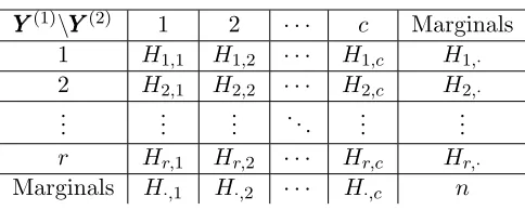
TABLE 2 : Contingency Table with Marginals. . . 126
LIST OF FIGURES
FIGURE 1 : Two models of adaptive data analysis. . . 6
FIGURE 2 : Interaction between analystAand datasetXXXvia algorithmsM1,· · ·,Mk. . . . 7
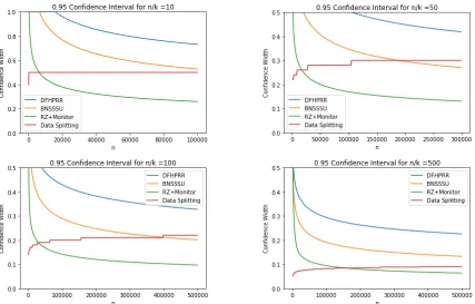
FIGURE 3 : Widths of valid confidence intervals forkadaptively chosen
statis-tical queries via data-splitting techniques or noise addition on the
same dataset. . . 41 FIGURE 4 : Standard deviations of the Gaussian noise we added to each query
to obtain the confidence widths. . . 42
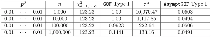
FIGURE 5 : Empirical Type I Error in 10,000 trials when using the classicalGOF
test without modification after incorporating noise due to privacy
for (= 0.1)-DP and (ρ=2/8)-zCDP. . . 118 FIGURE 6 : Empirical Type I Error ofAsymptGOFwith error bars corresponding
to 1.96 times the standard error in 100,000 trials. . . 134
FIGURE 7 : (Log of) Critical values of AsymptGOF and MCGOF (with m = 59)
with both Gaussian (ρ = 0.00125) and Laplace noise ( = 0.1) along with the classical critical value as the black line. . . 134
FIGURE 8 : Empirical Type I Error ofAsymptIndepwith error bars
correspond-ing to 1.96 times the standard error in 1,000 trials. . . 136
FIGURE 9 : Empirical Type I Error ofMCIndepusing Gaussian noise with error
bars corresponding to 1.96 times the standard error in 1,000 trials. 136
FIGURE 10 : Empirical Type I Error ofMCIndep using Laplace noise with error
FIGURE 11 : Comparison of empirical power of classical non-private test versus
AsymptGOF(solid line) andMCGOF(dashed line) with Gaussian noise for alternate H1 :ppp1 =ppp0+ ∆∆∆ in 10,000 trials. . . 137
FIGURE 12 : Comparison of empirical power of classical non-private test versus
MCGOFwith Laplace noise for alternate H1 :ppp1 =ppp0+ ∆∆∆ in 10,000
trials. . . 138 FIGURE 13 : Comparison of empirical power of classical non-private test versus
AsymptIndep(solid line) andMCIndep(dashed line) with Gaussian noise in 1,000 trials. . . 139
FIGURE 14 : Comparison of empirical power of classical non-private test versus
MCIndepwith Laplace noise in 1,000 trials. . . 140
FIGURE 15 : Empirical Type I Error for our goodness of fit tests inNewStatAsymptGOF
with the nonprojected statistic Q(ρn). . . 161
FIGURE 16 : Empirical Type I Error for our goodness of fit tests inNewStatAsymptGOF
with the projected statisticQ(ρn). . . 161 FIGURE 17 : Comparison of empirical power of classical non-private test versus
NewStatAsymptGOF with both projected (solid line) and
nonpro-jected statistics (dashed line). . . 163
FIGURE 18 : Comparison of empirical power between all zCDP hypothesis tests
for goodness of fit andNewStatAsymptGOF with projected statistic. 164
FIGURE 19 : Empirical Type I Error for our new independence tests inGenChiTest
with the nonprojected statistic. . . 169 FIGURE 20 : Empirical Type I Error for our new independence tests inGenChiTest
with the projected statistic. . . 169
FIGURE 21 : Comparison of empirical power of classical non-private test versus
FIGURE 22 : Comparison of empirical power between all zCDP hypothesis tests
for independence andGenChiTestwith projected statistic. . . . 171
FIGURE 23 : A comparison of empirical power between GenChiTest with
pro-jected statistic and output perturbation from Yu et al. (2014) for
independence testing for GWAS type datasets. . . 173
FIGURE 24 : Comparison of empirical power of classical non-private test versus
local private testsLocalGOF (solid line) and MC-GenChiTestwith
projected statistic and Laplace noise (dashed line) for alternate
H1 :ppp1 =ppp0+ ∆∆∆ in 1,000 trials. We setppp0 = (1/4,1/4,1/4,1/4)|
and H1:ppp0+ ∆∆∆ where ∆∆ = 0.01∆ ·(1,−1,−1,1)|. . . 182
FIGURE 25 : Comparison of empirical power of classical non-private test versus
local private testsLocalGOF (solid line) and MC-GenChiTestwith
Laplace noise and projected statistic (dashed line) in 1,000 trials.
List of Algorithms
1 MonitorWD[M,A](XXX) . . . 39
2 FixedParamComp(A,E, b) . . . 81
3 AdaptParamComp(A, k, b) . . . 82
4 PrivacyFilterComp(A, k, b;COMPg,δg) . . . 85
5 SimulatedComp(A, k, b) . . . 86
6 Stopping Time Adversary: A,δ . . . 99
7 Classical Goodness of Fit Test for Multinomial Data: GOF . . . 115
8 MC Private Goodness of Fit: MCGOF . . . 120
9 Private Chi-Squared Goodness of Fit Test: AsymptGOF . . . 123
10 Pearson Chi-Squared Independence Test: Indep. . . 127
11 Two Step MLE Calculation: 2MLE . . . 130
12 MC Independence Testing MCIndep . . . 131
13 Private Independence Test for r×ctables: AsymptIndep . . . 133
14 New Private Statistic Goodness of Fit Test: NewStatAsymptGOF . . . 156
15 Private General Chi-Square Test: GenChiTest. . . 167
16 Private Minimum Chi-Square Test using MC MC-GenChiTest . . . 174
17 Exponential MechanismMEXP . . . 179
18 Local DP GOF TestLocalGOF . . . 180
19 Local DP General Chi-Square Test LocalGeneral . . . 183
20 Local Randomizer MFC . . . 185
21 Extended Monitor WD[M,A](XXX) . . . .~ 194
22 First Algorithm in Lower Bound Construction: M1 . . . 199
Part I
PROBLEM STATEMENT AND
We first present the basic setup of adaptive data analysis including the motivation for why
analysts that depend on statistical findings should be concerned with it and what some of
the challenges are with adaptivity. We discuss some of the related work in this area, with
the first paper in this line of research being Dwork et al. (2015c), which will be crucial to
know when outlining our contributions. We then outline the rest of the dissertation, which
largely follows work previously published in Rogers et al. (2016a,b); Gaboardi et al. (2016); Kifer and Rogers (2016), but does contain some results not previously published.
Some preliminaries in differential privacy are then presented which will be needed
through-out the dissertation. We then conclude this first part of the thesis with empirical evaluations
of valid confidence bounds that we can generate for adaptively chosen statistical queries
us-ing previous results and a new analysis, which have not been compared before. This then
provides a link between the highly theoretical work in adaptive data analysis with some
CHAPTER 1
INTRODUCTION
The goal of statistics and machine learning is to draw conclusions on a dataset that will
generalize to the overall population, so that the same conclusion can be drawn from any new dataset that is collected from the same population. Tools from statistical theory have
become ubiquitous in empirical science stretching across a myriad of disciplines.
However, classical statistical tools are only useful insofar as the original theory was intended.
The scientific community has become increasingly aware that many of the “statistically
significant” findings in published research are frequently invalid. In many replication studies,
the published findings cannot be confirmed in a large proportion of them; much more than
would be allowed by the theory, e.g. Ioannidis (2005); Gelman and Loken (2014). When
a conclusion is made on a given dataset but cannot be replicated in other studies, then a
false discovery has been committed. Similarly, in machine learning, the validity of models are based on how well the model generalizes to new instances, with the main concern being
that the modeloverfits to the dataset and not the population.
Why is their an apparent disconnect between what theoretical statistics guarantees and
the overwhelming number of false discoveries that are made from empirical studies? One
of the crucial assumptions made in the classical theory is that the procedures that are
to be conducted on the dataset are all known upfront, prior to actually seeing the data.
In fact, one of the main suspects behind the prevalence of false discovery in replication
studies is that the data analyst is adaptively selecting different analyses to run based on previous results on the same dataset and using the classical theory as if the tests were
selected independently of the data (Gelman and Loken, 2014). This problem of adapting
“researcher degrees of freedom” (Ioannidis, 2005; Simmons et al., 2011; Gelman and Loken,
2014). As soon as the analyst has looked at the data or some function of it and then selects a
new analysis, the traditional theory is no longer valid. For example, it may be the case that
the analyst wishes to select some variables for a model selection followed by some inference
– note that the adaptive selection of the model invalidates the following inference using
classical statistical theory. Over the past few decades there has been a significant amount of effort put into proposing fixes to this problem. Despite some techniques for preventing
false discoveries, e.g. the Bonferroni Correction (Bonferroni, 1936; Dunn, 1961) and the
Benjamini-Hochberg Procedure (Benjamini and Hochberg, 1995), the problem still persists.
The practice of modern data analysis is inherently adaptive, where each analysis is
con-ducted based on previous outcomes on the same data as part of an exploratory analysis. It
may not be the case that a particular study would be thought of prior to running a test on
the data, thus making preregistering what analyses you want to run useless. Typically, an
analyst needs to use the data to find interesting analyses to perform and hypotheses to test. Further, as researchers increasingly allow open access of their data, multiple studies may
be conducted on the same dataset where findings of different research groups may influence
the studies performed by other research groups. Not taking into account the adaptivity
in the separate research groups’ analyses, this process can often lead to false conclusions
drawn from a dataset, thus contributing to the crisis in reproducibility.
In order to use classical techniques in this adaptive setting, we would require the analyst to
sample a fresh dataset with each new analysis to be conducted. Due to data collection being
costly, this is certainly not an ideal solution. Instead, we would like to be able to consider several, adaptively chosen analyses on the same dataset and ensure valid conclusions are
made that generalize to the population.
Recently, two lines of work have attempted to understand and mitigate the prevalence of
false discoveries in adaptive data analysis. The first is to derive tight confidence intervals
selection followed by regression (Fithian et al., 2014; Lee et al., 2013). The second line
of work originated in the computer science community by Dwork et al. (2015c) and seeks
to be very general by imposing conditions on the types of algorithms that carry out the
analysis at each stage and makes no assumption on how the results are used by the analyst.
Note that in the former line of work – called selective inference – the methods are focused
on two stage problems: variable selection followed by significance testing and adjust for the inference in the second step. The main idea of the latter line of work aims to limit the
amount ofinformation(a notion which we will make precise later) that is released about the
dataset with each analysis so that it is unlikely to commit a false discovery on a subsequent
analysis. This dissertation is largely a continuation of the work initiated by Dwork et al.
(2015c) and aims to further understand how we can correct for adaptivity in the classical
theory. We then present some useful hypothesis tests which can be used in this adaptive
setting while providing valid p-values.
Before we can discuss the specific contributions of this dissertation, we need to first discuss some of the previous work done in adaptive data analysis. We start by presenting a basic
setup of the problem so that we can discuss the difficulty that arises when we need to consider
analyses that are conducted adaptively on the same dataset as opposed to having the
analyses known upfront. We will then discuss further advances in understanding adaptive
data analysis and some of the results that have been shown.
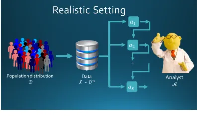
Throughout this dissertation, we will write the data universe as X, typically X = {0,1}d
where dis the dimensionality of the data, and some unknown data distribution D over X
where a datasetXXX = (X1,· · · , Xn) ofnsubjects is typically sampled i.i.d. fromD, denoted
asXXX ∼ Dn. The analyst’s goal is to infer something from the population rather than the
dataset. An analyst will then select a sequence of analyses that she wants to conduct,
receiving answers a1,· · · , ak that are computed using the dataset. Ideally, we would want
is used on. Realistically, due to data collection being costly, we would like to reuse the
same dataset for each analysis. See Figure 1 for a cartoon comparison between the ideal
and realistic settings of adaptive data analysis.
Analyst
𝒜
(a) The ideal setting – each analysis is per-formed on a fresh dataset.
(b) A more realistic setting – a single dataset is reused for adaptively chosen analyses.
Figure 1: Two models of adaptive data analysis.
1.1. Problem Formulation - Statistical Queries
We start by formulating the problem of adaptivity for a simple setting that is standard in
statistics and statistical learning theory, although later we will look at more general analyses
that the analyst can conduct on the data. Here, we address the problem where the analyst wants to know EX∼D[φ(X)] whereφ:X →[0,1]. For notational convenience we will write
this expectation as φ(D)defn= EX∼D[φ(X)]. The analyst then wants to obtain an estimate toφ(D) that is within tolerance τ with only access to sampled dataXXX∼ Dn.
This formulation of the problem is nice because this estimate is a statistical query in the
SQ model of Kearns (1993). We then model the interaction between an analystA wanting
to ask such queriesφi:X →[0,1] and algorithmsMi fori∈[k] which have direct access to
the datasetXXX∼ Dn. Here we model the analystAas first selectingφ
1 and receiving answer
a1=M1(XXX), then fori= 2,· · · , k, we allowAto selectφi as a function ofφ1,· · · , φi−1 and
answers a1,· · ·, ai−1 and she receives answer ai = Mi(XXX). Note that the algorithms Mi
is to report the empirical average,φi(XXX)defn= n1Pnj=1φi(Xi), which we know will be close to
φi(D) when φi are chosen independently of the data. Thus the analyst makes decisions on
what queries to ask based only on the outcomes of the algorithmsM1,· · ·,Mk. We then
outline this interaction so that for eachi∈[k] (also see Figure 2):
• AnalystA selects query φi, which is based on previous queriesφ1,· · · , φi−1 and
cor-responding answersa1,· · ·, ai−1
• A receives answer ai = Mi(XXX), where Mi may also depend on φ1,· · · , φi−1 and
a1,· · ·, ai−1.
Population distribution
! % ∼ !Data'
()
*)
(+
*+
(,
*,
⋮
Analyst 4
Figure 2: Interaction between analystA and datasetXXX via algorithms M1,· · · ,Mk. We then define what we mean by accuracy in this setting.
Definition 1.1.1. A sequence of algorithms M = (M1,· · ·,Mk) is (τ, β)-accurate with respect to the population if for all analysts A we have
Pr
max
i∈[k]|φi(D)− Mi(XXX)| ≤τ
≥1−β
where the probability is over the dataset XXX ∼ Dn as well as any randomness from the
Before we dive deeper into the adaptive setting, we first consider the case where all the
queries are asked up front, prior to any computations on the data. In this case we can
apply a Chernoff bound and union bound to show that releasing the empirical average on
the data is accurate,
Pr
XXX∼Dn
"
max
i∈[k]
|φi(D)−φi(XXX)| ≤
r 1
2nlog(2k/β) #
≥1−β
A useful quantity for comparing the different methods in this section will besample
complex-ity, which gives a bound on the sample size n that is sufficient in answeringknonadaptive
queries all with accuracy at mostτ with constant probability, sayβ = 0.05. Thus, answering
each (nonadaptively chosen) statistical query with the empirical average achieves sample
complexity n= Θ log(k)/τ2
.1 Phrased another way, we can answer an exponential inn number of statistical queries and still achieve high accuracy on all of them. Further, it is
a straightforward protocol that achieves this: simply answer with the empirical averages of
each statistical query. However, this analysis crucially requires the statistical queries all be
independent of the data.
We now consider the setting where the statistical queries are adaptively chosen. One first approach might be to just answer each statistical query with the empirical average, as we did
in the nonadaptive case. As pointed out in Hardt and Ullman (2014), we can use techniques
from Dinur and Nissim (2003) to nearly reconstruct the entire database after seeingO(τ2n) many random empirical averages to statistical queries (nonadaptively chosen), so that the
analyst can then find a statistical query q∗ such that |q∗(XX)X −q∗(D)| > τ with constant
probability. This translates to empirical averages only having sample complexity Ω(k/τ2). Thus, only a linear number of statistical queries can be answered accurately using empirical
estimates – an exponential blow up with a single round of adaptivity!
1Throughout the dissertation, we will use log(·) to denote the natural log unless we use another base, in
1.2. Prior Results - Statistical Queries
Given that empirical averages do not achieve good sample complexity with adaptively chosen
statistical queries, we hope to find new ways in which to answer these queries accurately.
There has then been a lot of work in developing algorithms that can answer much more
than a linear number of adaptively selected statistical queries. The following result, which
improves on an earlier result from Dwork et al. (2015c), shows that we can achieve a
quadratic improvement on the number of adaptively selected queries, using techniques from Dwork et al. (2006b), which we will extensively go over in Chapter 3.
Theorem 1.2.1[Bassily et al. (2016)]. There is an algorithm that has the following sample
complexity fork adaptively chosen statistical queries
n≥Oe
√
k τ2
!
.2
Further, the algorithm runs in time that is polynomial in n andlog|X | per query.
The following theorem, which also improves on an earlier result of Dwork et al. (2015c),
shows that we can accurately answer an exponential innnumber of adaptively selected
sta-tistical queries, but the algorithm which computes the answers is not run-time efficient. This
result follows from the Private Multiplicative Weights algorithm from Hardt and Rothblum
(2010).
Theorem 1.2.2[Bassily et al. (2016)]. There is an algorithm that has the following sample
complexity fork adaptively chosen statistical queries
n≥Oe p
log|X |log(k) τ3
!
.
Further, the algorithm runs in time that is polynomial in n and|X | per query.
An immediate question that arises when comparing these results is why the gap between
2We will use e
efficient and inefficient run-time algorithms (the second result requires |X |time per query)
when improving on sample complexity? There was no such distinction in the nonadaptive
setting. It turns out that this separation is actually inherent when answering adaptively
selected statistical queries accurately – adaptivity actually does come at a cost. The
follow-ing result was first studied in Hardt and Ullman (2014) who gave the first computational
barrier in answering adaptively selected queries and was then improved by Steinke and Ullman (2015).
Theorem 1.2.3 [Steinke and Ullman (2015)]. Under a standard hardness assumption,3
there is no computationally efficient algorithm that is accurate within constant tolerance
with constant probability (over randomness of the sample and the algorithm) on k=O(n2)
adaptively chosen statistical queries with X ={0,1}d.
It is worth pointing out here the dependence of this impossibility result on the dimensionality
of the data. Note that if n were much larger than 2d, then the empirical average of every
possible statistical query could be answered accurately. So for these results to be interesting, we are consideringn2d.
The gap between the upper and lower bounds in sample complexity for adaptively
cho-sen statistical queries is large. Hardt and Ullman (2014) and Steinke and Ullman (2015)
showed thatn=Oe
min{√k/τ,plog(|X |)/τ}samples are necessary forτ accuracy for k
adaptively chosen statistical queries.
Although in this section we focused entirely on statistical queries, it is possible to obtain
similar results for much richer classes of queries an analyst would like to ask about a dataset. Bassily et al. (2016) give results for the class of low sensitivity queries q:Xn→
R, defined
as functions where for any two neighboring datasets xxx, xxx0 ∈ Xn, that is xxx and xxx0 are the
same in every entry except one element, we have
|q(xxx)−q(xxx0)| ≤∆(q) =o(1) asn→ ∞.
We call ∆(q) thesensitivity of functionq. For the particular results in Bassily et al. (2016)
that we cite, we require ∆(q) = O(1/n), although their results do hold for more general
sensitivities.
1.3. Post Selection Hypothesis Testing
The goal of this dissertation is to handle much more general types of analyses, rather than
just statistical queries or low-sensitivity queries, in this adaptive setting. One specific type
of analysis we might like to handle adaptively is hypothesis testing. In fact, the previous
works (Dwork et al., 2015c; Bassily et al., 2016) are motivated by the problem of false
discovery in empirical science despite the technical results being about estimating means of
adaptively chosen statistical (or low-sensitivity) queries.
We will consider a simple model of one-sided hypothesis tests on real valued test statistics. A
hypothesis test is defined by atest statisticφ(j):Xn→
Rmapping datasets to a real value,
where we usejto index different test statistics. Given an outputa=φ(j)(xxx), together with
a distribution D over the data domain, the p-value associated with aand D is simply the
probability of observing a value of the test statistic that is at least as extreme asa, assuming
the data was drawn independently from D: p(Dj)(a) defn= PrXXX∼Dn[φ(j)(XXX) ≥ a]. Note that
there may be multiple distributionsDover the data that induce the same distribution over
the test statistic. With each test statistic φ(j), we associate a null hypothesis H(0j) as a collection of possible distributions overX. The p-values are always computed with respect
to a distribution D ∈ H(0j), and hence from now on, we hide the dependence on D and simply writep(j)(a) to denote the p-value of a test statistic φ(j) evaluated at a.
The goal of a hypothesis test is toreject the null hypothesis if the data is not likely to have
been generated from the proposed model, that is if the underlying distribution from which
the data were drawn was not in H(0j). By definition, ifXXX truly is drawn from Dn for some
value of the test statistic a = φ(j)(XX), and thenX reject the null hypothesis if p(j)(a) ≤ α. Under this procedure, the probability of incorrectly rejecting the null hypothesis—i.e., of
rejecting the null hypothesis whenXXX∼ Dn for someD ∈H(j)
0 —is at most α. Note that an
incorrect rejection of the null hypothesis is called afalse discovery.
The discussion so far presupposes that φ(j), the test statistic in question, was chosen in-dependently of the dataset XXX. Let Y denote a collection of test statistics, and suppose
that we select a test statistic using a data-dependent selection procedure M : Xn → Y.
If φ(j) = M(XXX), then rejecting the null hypothesis when p(j)(φ(j)(XXX))≤ α may result in a false discovery with probability much larger than α. As we mentioned earlier, this kind
of na¨ıve approach to post-selection inference is suspected to be a primary culprit behind
the prevalence of false discovery in empirical science (Gelman and Loken, 2014; Wasserstein
and Lazar, 2016; Simmons et al., 2011). This is because even if the null hypothesis is true
(XXX ∼ Dn for some D ∈ H(j)
0 ), the distribution onXXX conditioned on φ(j) =M(XXX) having
been selected need not beDn. Our goal in studying valid post-selection hypothesis testing is
to then find avalid p-value correction functionγ : [0,1]→[0,1], which we define as follows:
Definition 1.3.1[Validp-value Correction Function]. A functionγ : [0,1]→[0,1]is a valid
p-value correction function for a selection procedure M:Xn→ Y if for every significance
level α∈[0,1], the procedure:
1. Select a test statistic φ(j) =M(XXX) using selection procedure M. 2. Reject the null hypothesis H(0j) if p(j)(φ(j)(XXX))≤γ(α).
has probability at mostα of resulting in a false discovery.
We will be interested in p-value corrections that are not too small – note that γ(α) = 0 is
a valid correction but not very interesting. We would like our tests to be able to correctly
reject a wrong H(0j) with higher confidence as we increase the sample size. The ability for a hypothesis test to correct reject a null hypothesis is called the power of the test. We then
alternate hypothesis, different from the null. Typically in hypothesis testing, we want to
ensure the probability of a false discovery is at most some threshold α, and we would like
to minimize the probability of type II error, i.e. failing to reject when the null hypothesis
was false.
H(0j) True H(1j) True
Reject H(0j) False Discovery Power
Fail to Reject H(0j) Significance Type II Error
Table 1: Types of Errors in Hypothesis Testing
Necessarily, to give a nontrivial correction function γ, we will need to assume that the
selection procedure M satisfies some useful property. We will discuss later the types of
test selection procedures that will enable us to find valid correction functions. In
Ap-pendix A.1, we show that hypothesis testing is in general beyond the setting of statistical
or low-sensitivity queries that we have already discussed above, which shows that we need
new tools for handling adaptive hypothesis testing.
It is important to point out the role of the algorithm M : Xn → Y here. Before, we
were considering an algorithm that was given access to a dataset and would release answers
to adaptively chosen queries from the data analyst, then the analyst A would select any
new analysis (or query) based on the answers she had already witnessed. However, now
we are considering algorithms, or test selection procedures that release the analysis for the
analyst to use. This is simply for mathematical convenience. The seeming discrepancy
between these two models is resolved by the guarantees of the algorithms we will consider
here – that they are closed under post-processing. Thus, we can combine the output of the algorithm Mand the choice of analysis ofA as a single procedureM.
1.4. Handling More General Analyses - Max-information
There is one constraint on the selection procedureMthat does allow us to give nontrivial
Given two (arbitrarily correlated) random variables X, Z, we let X⊗Z denote a random
variable (in a different probability space) obtained by drawing independent copies ofX and
Z from their respective marginal distributions.
Definition 1.4.1 [Max-Information (Dwork et al., 2015a)]. Let X and Z be jointly
dis-tributed random variables over the domain (X,Z). The max-information between X and
Z, denoted by I∞(X;Z), is the minimal value ofm such that for every x in the support of X andz in the support ofZ, we have Pr [X=x|Z=z]≤2mPr [X =x]. Alternatively,
I∞(X;Z) = log2 sup (x,z)∈(X,Z)
Pr [(X, Z) = (x, z)] Pr [X⊗Z = (x, z)].
Theβ-approximate max-information betweenX and Z is defined as
I∞β (X;Z) = log2 sup
O⊆(X ×Z),
Pr[(X,Z)∈O]>β
Pr [(X, Z)∈ O]−β Pr [X⊗Z ∈ O] .
We say that an algorithm M:Xn→ Y has β-approximate max-information of m, denoted
asI∞β (M, n)≤m, if for every distributionSover elements ofXn, we haveI∞β (XXX;M(XXX))≤
m when XXX ∼ S. We say that an algorithm M : Xn → Y has β-approximate
max-information ofm over product distributions, written I∞β,Π(M, n)≤m, if for every distri-bution D over X, we have I∞β (XXX;M(XXX))≤m whenXXX ∼ Dn.
Max-information has several nice properties that are useful in adaptive data analysis. The
first is that it composes, so that if an analyst uses an algorithm with bounded approxi-mate max-information and then based on the output uses another algorithm with bounded
approximate max-information, then the resulting analysis still has bounded approximate
max-information.
Theorem 1.4.2 [Dwork et al. (2015a)]. Let M1 : Xn → Y be an algorithm such that
Iβ1
∞(M1, n) ≤ m1 and let M2 : Xn× Y → Z be an algorithm such that for each y ∈ Y,
we have Iβ2
∞(M2(·, y), n). Then the composed algorithm M : Xn → Z where M(xxx) =
thenIβ1+β2
∞,Π (M, n)≤m1+m2
Note that this result can be iteratively applied to string together a sequence of adaptively
chosen algorithms with approximate max-information and the resulting composed algorithm
will also have bounded max-information. This composition theorem is crucial in
control-ling the probability of false discovery over a sequence of analyses when each analysis is individually known to have bounded max-information.
Another useful property is that max-information is preserved under post-processing. Thus,
if our algorithmManswers adaptively chosen analyses (e.g. statistical queries) on dataset
XXX and has bounded approximate max-information, then the analyst can take any function
of the output f(M(XXX)) =M0(XXX) to find a new analysis to run. The resulting algorithm
M0 then has max-information bound no larger than that ofM.
Theorem 1.4.3 [Dwork et al. (2015a)]. If M:Xn → Y and ψ :Y → Y is any (possibly
randomized) mapping, thenψ◦ M:Xn→ Y0 satisfies the following for any random variable XXX over Xn and every β ≥0,
I∞β (XXX;ψ(M(XXX)))≤I∞β (XXX;M(XXX)).
We now state some of the immediate consequences of max-information in adaptive data
analysis. It follows from the definition that if an algorithm has bounded max-information,
then we can control the probability of “bad events” that arise as a result of the dependence of
M(XXX) onXXX: for every eventO, we have Pr[(XXX,M(XXX))∈ O]≤2mPr[XXX⊗ M(XXX)∈ O] +β.
For example, if Mis a data-dependent selection procedure for selecting a test statistic, we
can derive a valid p-value correction function γ as a function of a max-information bound on M:
correction function for M:
γ(α) = max
α−β 2m ,0
.
Proof. Fix a distributionD from which the datasetXXX∼ Dn. If α−β
2m ≤0, then the theorem
is trivial, so assume otherwise. Define O ⊂ Xn× Y to be the event thatM selects a test
statistic for which the null hypothesis is true, but itsp-value is at mostγ(α):
O={(xxx, φ(j)) :D ∈H(0j) and p(j)(φ(j)(xxx))≤γ(α)}
Note that the event O represents exactly those outcomes for which using γ as a p-value
correction function results in a false discovery. Note also that, by definition of the null
hypothesis, Pr[XXX⊗M(XXX)∈ O]≤γ(α) = α2−mβ. Hence, by the guarantee thatI β
∞,Π(M, n)≤
m, we have that Pr[(XXX,M(XXX)∈ O)] is at most 2m·α2−mβ
+β=α.
We can also use algorithms with small max-information to answer adaptively chosen
low-sensitivity functions, using McDiarmid’s inequality (given in Theorem A.1.1 in the
ap-pendix).
Theorem 1.4.5 [Dwork et al. (2015a)]. Let M: Xn → Y be a data-dependent algorithm
for selecting a function with sensitivity∆andI∞β,Π(M, n)≤log2(e) τ2/∆2
, then we have
for q =M(XXX) whereXXX ∼ Dn
Pr
X X
X,M[|q(D
n)−q(XXX)| ≥τ]≤exp
−τ2
n∆2
+β.
Max-information provides the correction factor in which we need to modify our analyses for
the dependence on the data. Up to the correction factor, we can then use existing statistical
1.5. Algorithms with Bounded Max-information
Due to Theorems 1.4.4 and 1.4.5, we are then interested in finding test selection procedures
M that have bounded approximate max-information. From Dwork et al. (2015a), there
are two families of algorithms which are known to have bounded max-information, which
we will discuss in turn. Note that these algorithms were known previously to give good
generalization guarantees for adaptively chosen analyses, but the two are otherwise
incom-parable. Thus, max-information can be seen as a unifying measure for different types of analyses which have good generalization guarantees.
We first state the result that gives us a max-information bound in terms of the description
length of the output ofM.
Theorem 1.5.1 [Dwork et al. (2015a)]. Let M:Xn → Y be a randomized algorithm with
finite output set Y. Then for each β >0, we have
I∞β (M, n)≤log2(|Y|/β).
We can interpret this result as saying that the shorter the result of an analysis, the better it
is for adaptive data analysis settings because it reveals less information about the dataset
and leads to better generalization for subsequent analyses.
The second type of algorithms that were known to have bounded max-information are (pure)
differentially private algorithms. At a high level, differential privacy is a stability guarantee
on an algorithm in that it limits the sensitivity of the outcome to any individual data
entry from an input dataset. Although differential privacy was introduced for private data
analysis applications (Dwork et al., 2006b), where the dataset is assumed to contain sensitive
information about its subjects, we can leverage the stability guarantees of differential privacy
to answer new questions in various problems beyond privacy concerns. In fact, differential
2016b, 2015; Kannan et al., 2015). Similarly, differential privacy has been shown to be a
useful tool in adaptive data analysis (Dwork et al., 2015c,a; Bassily et al., 2016), which is
the connection we explore in this dissertation.
We will give the definition and useful properties of differential privacy in Chapter 2, but we
state here the bound on max-information.
Theorem 1.5.2 [Pure Differential Privacy and Max-Information (Dwork et al., 2015a)].
Let M:Xn→ Y be an(,0)-differentially private algorithm. Then for every β >0:
I∞(M, n)≤log2(e)·n and I∞,Π(M, n)≤log2(e)·
2n/2 +pnln(2/β)/2
Due to the composition property of max-information in Theorem 1.4.2, we can string pure
differentially private algorithms together with bounded description length algorithms in
arbitrary orders and still obtain generalization guarantees for the entire sequence.
The connection in Theorem 1.5.2 is powerful, because there are a vast collection of data
analyses for which we have differentially private algorithms, including a growing literature – some which we will cover in this dissertation – on differentially private hypothesis tests
(Johnson and Shmatikov, 2013; Uhler et al., 2013; Yu et al., 2014; Karwa and Slavkovi´c,
2016; Dwork et al., 2015d; Sheffet, 2015b; Wang et al., 2015; Gaboardi et al., 2016; Kifer and
Rogers, 2016). However, there is an important gap: Theorem 1.5.2 holds only forpure(,
0)-differential privacy, and not for the broader class, (approximate) (, δ)-0)-differential privacy,
where δ > 0. Many statistical analyses can be performed much more accurately subject
to approximate differential privacy, and it can be easier to analyze private hypothesis tests
that satisfy approximate differential privacy, because the approximate privacy constraint
is amenable to perturbations using Gaussian noise (rather than Laplace noise) (Gaboardi et al., 2016; Kifer and Rogers, 2016). Most importantly, for pure differential privacy, the
approximate differential privacy,need only degrade with thesquare root of the number of
analyses performed (Dwork et al., 2010). Hence, if the connection between max-information
and differential privacy held also for approximate differential privacy, it would be possible to
perform quadratically more adaptively chosen statistical tests without requiring a smaller
p-value correction factor. In fact, for the sample complexity results given in Theorems 1.2.1
and 1.2.2, in order to answer k adaptively chosen statistical queries accurately, we require that the overall composed algorithmMk◦ · · · ◦ M1 be approximately differentially private.
1.6. Contributions
We are now ready to discuss the specific contributions of this dissertation in understanding
adaptive data analysis.
We will first demonstrate how we can use the previous results in adaptive data analysis
for obtaining valid confidence intervals on adaptively chosen statistical queries using results from Dwork et al. (2015c), Bassily et al. (2016), and Russo and Zou (2016). Although, we
know that we can asymptotically outperform data-splitting techniques, we show in
Chap-ter 3 that we can improve even for reasonably sized datasets.
In Chapter 4 we extend the connection between differential privacy and max-information
to approximate differential privacy, which follows from work published by Rogers et al.
(2016a). We show the following (see Section 4.2 for a complete statement):
Theorem 4.2.1 (Informal). Let M : Xn → Y be an (, δ)-differentially private
algo-rithm. Then,
I∞β,Π(M, n) =Oe
n2+n q
δ
forβ=Oe
n q
δ
.
It is worth noting several things. First, this bound nearly matches the bound for
rithms. The bound is qualitatively tight in the sense that despite its generality, it can be
used to nearly recover the tight bound on the generalization properties of differentially
pri-vate mechanisms for answering low-sensitivity queries that was proven using a specialized
analysis in Bassily et al. (2016), see Section 4.3 for a comparison.
We also only prove a bound on the max-information for product distributions on the input, and not for all distributions (that is, we bound I∞β,Π(M, n) and not I∞β (M, n)). A bound for general distributions would be desirable, since such bounds compose, see Theorem 1.4.2.
Unfortunately, a bound for general distributions based solely on (, δ)-differential privacy is
impossible: a construction inspired by work from De (2012) implies the existence of (,
δ)-differentially private algorithms for which the max-information between input and output
on arbitrary distributions is much larger than the bound in Theorem 4.2.1.
One might nevertheless hope that bounds on the max-information under product
distribu-tions can be meaningfully composed. Our second main contribution is a negative result, showing that such bounds do not compose when algorithms are selected adaptively.
Specif-ically, we analyze the adaptive composition of two algorithms, the first of which has a small
finite range (and hence, by Dwork et al. (2015a), small bounded max-information), and the
second of which is (, δ)-differentially private. We show that the composition of the two
al-gorithms can be used to exactly recover the input dataset, and hence, the composition does
not satisfy any nontrivial max-information bound. We then draw a connection between
max-information and Shannon mutual information that allows us to improve on several
prior results that dealt with mutual information in McGregor et al. (2011) and Russo and
Zou (2016).
An important feature of differential privacy is that it is preserved under composition, that
is combining many differentially private subroutines into a single algorithm preserves
dif-ferential privacy and the privacy parameters degrade gracefully. However, there is a caveat
to these composition theorems. In order to apply these results from differential privacy, we
data. In Chapter 5, we then give a framework for composition that allows for the types of
composition theorems of differential privacy to work in this adaptive setting, which follows
from work by Rogers et al. (2016b). We give a formal separation between the standard
model of composition and our new setting, so that we cannot simply plug in the adaptively
chosen privacy parameters into existing differential privacy composition theorems as if the
realized parameters were fixed prior to running any analysis. Despite this result, we still give a bound on the privacy loss when the parameters can be adaptively selected which
for datasets of size n is asymptotically no larger than √log logn times the bound from
the advanced composition theorem of Dwork et al. (2010), which assumes that the privacy
parameters were selected beforehand.
After understanding the benefits of differential privacy in adaptive data analysis and how
composition may be applied in this setting, we then present in Chapters 6 and 7 some
primitives that an analyst may want to use at each round of interaction with the dataset.
Specifically we give hypothesis tests that ensure statistical validity while satisfying differen-tial privacy, focusing on categorical data and chi-square tests, such as tests for independence
and goodness of fit. Chapter 6 follows from work by Gaboardi et al. (2016) and Chapter 7
is from Kifer and Rogers (2016).
1.6.1. New Results
For the reader that is interested in results that are not publised elsewhere, we outline the
new contributions of this dissertation here:
• Chapter 3, which demonstrates the improvements we can obtain over data-splitting
techniques for computing confidence intervals on adaptively chosen statistical queries,
is new and based on ongoing work with Aaron Roth, Adam Smith, and Om Thakkar.
• We give a new implication of our lower bound result from Rogers et al. (2016a) in
• We show in Section 4.7 that procedures with bounded max-information are not
neces-sary to ensure generalization guarantees in the adaptive setting. Specifically, we show
that compression schemes can have arbitrarily large max-information.
• We use a different concentration bound (Theorem 5.4.2) from the one used in Rogers
et al. (2016b) to obtain a privacy odometer with better constants than what appeared in Rogers et al. (2016b), which then follows from a more simplified analysis, presented
in Theorem 5.6.5
• Section 5.7 extends privacy odometers and filters to include concentrated differentially
private algorithms, which were defined by Bun and Steinke (2016).
• All of the experiments in Part III have been redone so that it is easier to directly
compare empirical results of the different private hypothesis tests we propose.
• We give the variance of each of the chi-square statistics we consider in Theorem 7.2.12.
This gives a more analytical reason for why some tests achieve better empirical power
than others.
• We also give preliminary results on private hypothesis tests in the local model in
Chapter 8, where each individual’s data is reported in a private way, rather than in
the traditionalcurator setting which assumes there is a trusted curator that collects
everyone’s raw data.
1.7. Related Work
This dissertation follows a line of work that was initiated by Dwork et al. (2015c) and Hardt
and Ullman (2014), who formally modeled the problem in adaptive data analysis. Since
these works, there has been several other contributions (Dwork et al., 2015a,b; Bassily et al.,
2016; Russo and Zou, 2016; Cummings et al., 2016a; Wang et al., 2016), some in which we
have already discussed many of their results. We then use this section to discuss some of
One of the crucial observations of Dwork et al. (2015c) is that algorithms that are stable,
i.e. differentially private, can be leveraged to obtain strong generalization guarantees in
adaptive analysis. Stability measures the amount of change in the output of an algorithm
if the input is perturbed. Another line of work (Bousquet and Elisseeff, 2002; Mukherjee
et al., 2006; Poggio et al., 2004; Shalev-Shwartz et al., 2010) had established the connections
between stability of a learning algorithm and its ability to generalize, although in nonadap-tive settings. The problem with the stability notions that they consider is that they are
not robust to post-processing or adaptive composition. That is, if individual algorithms
are stable and known to generalize, then it is often not the case that stringing together a
sequence of these algorithms will still ensure generalization. The main benefit of the type
of stability that Dwork et al. (2015c) considers is that it is preserved under the operations
of post-processing and adaptive composition.
Russo and Zou (2016) consider different types of exploratory analyses through the lens of
information usage, similar to Dwork et al. (2015a). They study the bias that can result in adaptively chosen analyses, which are based on subgaussian statistics under the data
distribution. They prove that the bias can be bounded by the dependence between the
noise in the data and the choice of reported result using Shannon mutual information. To
obtain the type of generalization bounds that we are concerned with – high probability
guarantees – we can then apply Markov or Chebyshev’s inequality. We compare some of
our results with those of Russo and Zou (2016) in Section 4.6.
In a more restrictive setting, Wang et al. (2016) assumes that the analyst is selecting
statis-tics which are jointly Gaussian. They show that adding Gaussian noise to the statisstatis-tics is optimal in aminimax framework of adaptive data analysis. However, we are after generality
of analyses, which comes at the cost that our results might be overly conservative.
In order to perform many adaptively chosen analyses and ensure good generalization over
properties are known to hold already. Cummings et al. (2016a) then give three notions of
generalizations that are closed under post-processing and amendable to adaptive
composi-tion, with each strictly stronger than the next: robust generalizacomposi-tion, differential privacy,
and perfect generalization. Although bounded description length and differentially
pri-vate algorithms were known to be robustly generalizing, they demonstrate a third type –
compression schemes – that also gives guarantees of robust generalization.
There have also been successful implementations of algorithms that guard against overfitting
in adaptive data analysis. Specifically, Blum and Hardt (2015) gives a natural algorithm
– the Ladder – to ensure that a leaderboard is accurate in machine learning competitions
even when entries are allowed to evaluate their models several times on a holdout set,
each time making modifications based on how they may rank on the leaderboard. They
show that they can ensure a leaderboard accurately ranks the participants’ models despite
the adaptivity in real submission files and even give empirical results using real data from
the Kaggle competition. Additionally, Dwork et al. (2015a,b) show how their methods can reduce overfitting to a holdout set, using the algorithm they call Thresholdout, when
CHAPTER 2
PRIVACY PRELIMINARIES
We use this section to present what has become the standard privacy benchmark,differential
privacy, and then the more recent version calledconcentrated differential privacy. We then give some definitions and results that will be crucial for the rest of the dissertation.
We will define differential privacy in terms of indistinguishability, which measures the
sim-ilarity between two random variables.
Definition 2.0.1 [Indistinguishability (Kasiviswanathan and Smith, 2014)]. Two random
variablesX, Y taking values in a setX are (, δ)-indistinguishable, denoted X≈,δ Y, if for
allS ⊆ X,
Pr [X ∈S]≤e·Pr [Y ∈S] +δ and Pr [Y ∈S]≤e·Pr [X∈S] +δ.
2.1. Differential Privacy
Recall that when we defined sensitivity of a function, we say that two datasets xxx =
(x1,· · · , xn), xxx0 = (x10,· · · , x0n) ∈ Xn are neighboring if they differ in at most one entry,
i.e. there is some i∈[n] wherexi 6=x0i, butxj =x0j for allj 6=i.
Definition 2.1.1 [Differential Privacy (Dwork et al., 2006b,a)]. A randomized algorithm
(or mechanism) M : Xn → Y is (, δ)-differentially private (DP) if for all neighboring
datasetsxxx andxxx0 and each outcome S ⊆ Y, we have M(xxx)≈,δ M(xxx0) or equivalently
Pr [M(xxx)∈S]≤ePr
M(xxx0)∈S
+δ.
DP.
Note that in the definition, the data is not assumed to be coming from a particular
distribu-tion. Rather, the probability in the definition statement isonly over the randomness from
the algorithm. In order to compute some statisticf :Xn→
Rdon the data, a differentially
private algorithm is to simply add symmetric noise to f(xxx) with standard deviation that depends on theglobal sensitivity off, which we define as
∆p(f) = max
neighboringxxx,xxx0∈Xn{||f(xxx)−f(xxx
0)||
p}. (2.1)
We then give a commonly used differentially private algorithm, called the Laplace
Mecha-nism, which releases an answer to a query on the dataset with appropriately scaled Laplace
noise.
Theorem 2.1.2 [Laplace Mechanism (Dwork et al., 2006b)]. Let f : Xn →
Rd. The
algorithmM(xxx) =f(xxx) +LLL whereLLLi.i.d.∼ Lap(∆1(f)/), is -DP.
A very useful fact about differentially private algorithms is that one cannot take the output
of a differentially private mechanism and perform any modification to it that does not
depend on the input itself and make the output any less private. This is precisely the same property that max-information enjoys in Theorem 1.4.3.
Theorem 2.1.3 [Post Processing (Dwork et al., 2006b)]. Let M :Xn → Y be (, δ)-DP
andψ:Y → Y0 be any function mapping to arbitrary domainY0. Thenψ◦ M is(, δ)-DP.
One of the strongest properties of differential privacy is that it is preserved underadaptive
composition. That is, combining many differentially private subroutines into a single
algo-rithm preserves differential privacy and the privacy parameters degrade gracefully. We will
discuss in Chapter 5 a caveat to these composition theorems and propose a new framework
of composition, where the privacy parameters themselves may also be chosen adaptively.
Adaptive composition of algorithms models the way in which an analyst would interact
outcomes. We formalizeadaptive composition in the following way:
• M1:Xn→ Y1.
• For eachi∈[k], Mi:Xn× Y1× · · · × Yi−1 → Yi.
We will then denote the entire composed algorithm asM1:k:Xn→ Yk.
We first state a basic composition theorem which shows that the adaptive composition
satisfies differential privacy where “the parameters just add up.”
Theorem 2.1.4 [Basic Composition (Dwork et al., 2006b,a)]. Let each Mi : Xn× Y
1×
· · · × Yi−1 be (i, δi)-DP in its first argument for i∈[k]. ThenM1:k:Xn → Yk is (g, δg)
-differential privacy where
g = k
X
i=1
i, and δg= k
X
i=1
δi.
We now state the advanced composition bound originally given in Dwork et al. (2010) which
gives a quadratic improvement to the basic composition bound. We state the bound as given
by Kairouz et al. (2015), with improved constants and generalized it so that all the privacy
parameters need not be the same.
Theorem 2.1.5 [Advanced Composition (Dwork et al., 2010; Kairouz et al., 2015)]. Let
each Mi : Xn × Y
1 × · · · × Yi−1 be (i, δi)-DP in its first argument for i ∈ [k]. Then
M1:k:Xn→ Y
k is (g, δg)-differential privacy where for any bδ >0
g = k
X
i=1
i
ei−1
ei+ 1
+
v u u t2
k
X
i=1
2
i log(1/bδ), and δg = 1−(1−bδ)
k
Y
i=1
(1−δi).
privacy parameters (1, δ1),· · · ,(k, δk) andδg >0, find the best possible privacy parameter
g, so that any adaptive composition ofM1:k, where each algorithm is (i, δi)-DP fori∈[k]
is (g, δg)-DP.
We then define the privacy loss random variable, which quantifies how much the output
distributions of an algorithm on two neighboring datasets can differ.
Definition 2.1.6 [Privacy Loss]. Let M :Xn → Y be a randomized algorithm. We then
define the privacy loss variablePrivLoss (M(xxx)||M(xxx0))for neighboring datasetsxxx, xxx0 ∈ Xn
in the following way: let Z(y) = logPr[Pr[MM((xxxxxx0)=)=yy]]
and then PrivLoss (M(xxx)||M(xxx0)) is
distributed the same as Z(M(xxx)).
Note that if we can bound the privacy loss random variable with certainty over all
neigh-boring datasets, then the algorithm is pure DP. Otherwise, if we can bound the privacy loss
with high probability then it is approximate DP (see Kasiviswanathan and Smith (2014)
for a more detailed discussion on this connection). It is worth pointing out that the privacy loss random variable is central to proving Theorem 2.1.5 from Dwork et al. (2010).
2.2. Concentrated Differential Privacy
We will also use in our results a recently proposed definition of privacy calledzero
concen-trated differential privacy (zCDP), defined by Bun and Steinke (2016) (Note that Dwork
and Rothblum (2016) initially gave a definition of concentrated differential privacy which
Bun and Steinke (2016) then modified).
Definition 2.2.1 [zCDP]. An algorithm M:Xn→ Y is(ξ, ρ)-zero concentrated
differen-tially private (zCDP), if for all neighboring datasets xxx, xxx0 ∈ Xn and all λ >0 we have
Eexp λ PrivLoss M(xxx)||M(xxx0)−ξ−ρ≤eλ
2ρ
.
Typically, we will write (0, ρ)−zCDP simply as ρ-zCDP.