R E S E A R C H
Open Access
An efficient admission control model based on
dynamic link scheduling in wireless mesh
networks
Juliette Dromard
*, Lyes Khoukhi and Rida Khatoun
Abstract
Background: Wireless mesh networks (WMNs) are a very attractive new field of research. They are low cost, easily deployed, and a high-performance solution to last-mile broadband Internet access. In WMNs, admission control (AC) is one of the key traffic management mechanisms that should be deployed to provide quality of service (QoS) support for real-time traffic.
Results: In this paper, we introduce a novel admission control model, based on bandwidth and delay parameters, which integrates a dynamic link scheduling scheme. The proposed model is built on two different methods to access the medium: on a contention-based channel access method for control packets and on a dynamic time division multiple access (DTDMA) for data packets. Each time a new flow is admitted in the network, the WMN’s link scheduling is modified according to the flows’ requirement and network conditions while respecting the signal-to-interference-plus-noise ratio (SINR); this allows establishing collision-free transmissions.
Conclusions: Using extensive simulations, we demonstrate that our model achieves high resource utilization by improving throughput, establishing collision-free transmission, as well as respecting requirements of admitted flows in terms of delay and bandwidth.
Keywords: Wireless mesh networks; Admission control; Link scheduling
1 Introduction
Wireless mesh networks (WMNs) are autonomous net-works, made up of mesh routers and mesh clients, where mesh routers have minimal mobility and form the back-bone of WMNs. The bridge between the backback-bone mesh and other networks (e.g., Internet, cellular and sensor net-works, etc.) is achieved through gateways. Mesh routers relay the data injected by mesh clients in a multihop
ad hocfashion until reaching a gateway. WMNs are low cost, easily deployed, self-configuring, and self-healing and enable ubiquitous wireless access. Indeed, they can extend Internet access in areas where cable installation is impossible or economically not sustainable such as hostile areas, battlefields, old buildings, rural areas, etc. [1].
However, due to a lack of centralized management, unfairness between flows created by the contention-based channel access, and unreliable wireless channels, the
*Correspondence: [email protected]
University of Technology of Troyes, 12 rue Marie Curie, Troyes 10000, France
capacity of WMNs is limited. The capacity of a node tends to decrease with the number of hops which separates it from the gateway; this fact compromises the scalability of WMNs. Indeed, the throughput of each node decreases as
O(1/n), wherenis the total number of nodes in the
net-work [2]. That is why many applications with very strict constraints (e.g., VOIP and video streaming) cannot be deployed easily.
In order to solve the deployment issues of flows with very strict requirements in WMNs, several admission control (AC) schemes have been proposed in the literature [3-7]. AC schemes aim at guaranteeing flows’ constraints in WMNs by accepting a new flow on the backbone mesh only if the latter is able to guarantee its quality of ser-vice (QoS) and the QoS of previously accepted flows. Note that most existing ACs in WMNs are based on a contention-based channel access method, carrier sense multiple access with collision avoidance (CSMA/CA) [6]. CSMA/CA was originally built for infrastructure wireless
networks and turns out to be inappropriate in a multi-hop wireless network as it leads to low throughput and unfairness between nodes in WMNs [8].
To overcome the above limitations, several articles (e.g., [9-12]) propose to replace CSMA/CA by TDMA in WMNs. As TDMA is not a competition access scheme, it does not need methods to avoid collision (such as the backoff algorithm used in CSMA/CA) and can, thus, gain in throughput [12,13]. Furthermore, as it divides the access to the channel in time in order to avoid collisions, it also enables to limit packet loss rate [14]. However, in most existing TDMA schemes in WMNs, the applied link scheduling is fixed at the design stage of the network and does not evolve according to the traffic load; this may lead to network congestion. To alleviate these limitations, this paper proposes a novel admission control model based on dynamic link scheduling, which integrates bandwidth and delay as parameters. We note that a preliminary version of this work was published in [15]. Our model includes the following contributions:
• The use of the signal-interference-plus-noise-ratio (SINR) as the interference model in our AC. While most existing AC models (e.g., [4,5,16]) rely on either hop-based or distance-based interference model, our AC considers a more accurate interference model [17]: the SINR-based interference model. This allows establishing interference-free transmissions and increasing network throughput.
• An analytical formulation which allows computing the delay of any flow, knowing its scheduling over links it crosses. Integrated in an AC scheme, the latter accepts a flow only if its link scheduling respects the required delay. Furthermore, our analytical
formulation can be integrated in the IEEE 802.11s mesh coordination function controlled channel access (MCCA) [18] in order to ensure that the flows’ delay requirement is respected.
• A heuristic algorithm which allows dynamic link scheduling which respects traffic constraints in terms of delay and bandwidth. While most existing link scheduling solutions based on the SINR model do not consider dynamic traffic load in the network and propose fixed link scheduling, our algorithm updates link scheduling dynamically according to flows’ requirements and traffic load; this prevents the network from congestion.
To the best of our knowledge, it is the first time that an AC scheme considers dynamic link scheduling based on the SINR interference model. Our solution allows to over-come the lack of throughput of existing ACs in WMNs as well as the lack of traffic adaptation according to the network’s load and traffic types. The rest of the paper is
organized as follows. In Section 2, we survey recent works related to link scheduling and admission control schemes and underline the necessity to integrate AC and link scheduling schemes into a unique solution. In Section 3, we present our system model and formulate our prob-lem. In Section 4, we detail our proposed model. Section 5 evaluates the proposed admission control via simulations. Finally, Section 6 concludes this paper.
2 Related works
Several papers have addressed the problem of link scheduling to guarantee collision-free transmission. To deploy a link scheduling scheme in a WMN, the nodes must be synchronized and time must be divided into frames split into slots. Link scheduling schemes aim at selecting for each link in the network the slots in a frame during which the link is periodically activated while ensuring interference-free transmission and a maximum throughput in the network [14]. To avoid collisions, a link scheduling scheme should employ an interference model in order to establish which set of links can be activated simultaneously without causing any interference issue. The problem of link scheduling with the objec-tive of maximizing the network throughput is known to be NP-hard, even with a simple interference model [12]. Thus, most existing works propose heuristic algorithms which produce close-to-optimal (sub-optimal) solutions. The efficiency of a sub-optimal algorithm is typically mea-sured in terms of computational complexity (run time) and approximation factor (performance guarantee) [14]. Link scheduling schemes can be classified according to the interference model they are based on, which can be either a hop-based (e.g., [12,19]), a distance-based (e.g., [20,21]), or a SINR-based interference model (e.g., [10,22-24]).
In the hop interference model, a node can transmit
suc-cessfully if no node, situated atk-hops or more from it, is
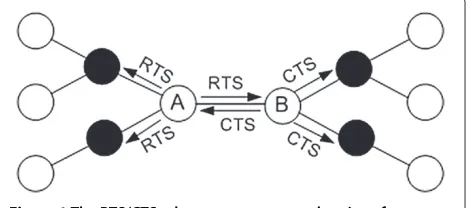
activated at the same time [25]. For example, the request to send/clear to send (RTS/CTS) scheme respects the one-hop interference model. Indeed, to transmit data over a link, the sender and the receiver of the link must previ-ously send RTS/CTS packets. Nodes situated at one hop of the sender or of the receiver which receives either a RTS or a CTS packet are then blocked to prevent interference during the link transmission. Figure 1 represents this phe-nomenon; it shows that if link A-B is active, the RTS/CTS scheme blocks the neighboring nodes (nodes in black) of node A and node B in order to avoid collisions.
In [10], the authors formulate the k-hop interference
model as ak-valid matching problem in a network graph.
They propose a scheduling scheme based on a greedy algorithm which computes sets of independent
maxi-mum k-valid matchings in the network graph. A
max-imum k-valid matching is the maximum set of edges
Figure 1The RTS/CTS scheme ensures a one-hop interference model.Nodes in black are blocked and cannot accept or launch any transmission.
can be activated simultaneously during some slot(s). The
algorithm searches for maximum k-valid matchings in
order to optimize the network throughput. However, this solution can only be deployed to a limited number of topology.
The authors in [19] consider the problem of scheduling the links of a set of routes in a WMN while respecting the hop-based interference model and maximizing the net-work throughput. In their approach, an undirected graph
Gis built where each node represents a link to schedule;
an edge may exist between two nodes if the links rep-resented by these nodes interfere with each other when they are activated simultaneously. The authors show that the problem of scheduling the links of a set of routes can be considered as a problem of multicoloring the nodes
of the graphG. They introduce two multicoloring-based
heuristics in order to schedule the links of the WMN and study their performance. However, the scalability aspect is not respected in their approach because they only study WMNs made up of a few nodes.
In a distance-based model, a transmission is successful if the distance between a receiver and a transmitter is less
or equal to the communication rangeRcand if no other
node is transmitting in the interference range Ri of the
receiver; i.e., within a distanceRifrom the receiver [17,20]
(see Figure 2).
In [21], the authors propose new methods for computing upper and lower bounds on the optimal throughput for any given network and workload. They also introduce a conflict graph model based on the distance-based interference model to represent clearly interferences between links. In their proposed conflict
graphF(V,E), each nodevi∈Vof the conflict graph
rep-resents a direct link in the network. The model assumes
that there exists an edgee=(vi, vj)withe∈Ewhich joins
up two links represented by nodesviandvj, if these two
links interfere with each other when they are activated simultaneously according to the distance-based interfer-ence model. The developed methods to compute upper and lower bounds on the optimal throughput assume that packet transmissions at the individual nodes can be finely
Figure 2Communication rangeRcand interference rangeRiof a
link A-B using the distance-based interference model.
controlled and carefully scheduled by an omniscient and omnipotent central entity, which is clearly unrealistic.
In [24], the authors investigate the problem of finding the link scheduling for a set of paths in a WMN relying on the distance based-interference model. They represent the issue by a mixed integer-nonlinear problem and pro-pose heuristics based on Lagrangian decomposition to compute suboptimal solutions. They show that their solu-tion is sub-optimal and can be rapidly computed in large WMNs. However, the interference model used in their solution is not the most realistic one and may lead to interference issues [26].
The SINR-based interference model assumes that a receiver successfully receives data if its SINR is greater than or equal to a certain threshold whose value can be given as physical layer properties of the network card [14]. The SINR-based model is not a local concept; indeed, any far away node can be involved in corrupting a transmis-sion [23]. So the SINR-based model is less restrictive and more accurate than both the hop-based or distance-based models; however, it is more complex.
In [10], the authors present a centralized polynomial time algorithm for link scheduling using the SINR-based interference model. This algorithm schedules link by link; each link is scheduled at slots such that the resulting sets of scheduled transmission are feasible. To maximize the network throughput, this algorithm looks at
mini-mizing schedule length (i.e., finding the shortest frame
relative to the shortest schedule possible under the SINR-based interference model. In their solution, the authors
assume that flows’ demands are known a prioriby the
scheduling module, which is an unrealistic assumption. In [22], the authors study the limits of the distance-based interference model and propose a conflict-free link scheduling algorithm (CFLS) based on the Matroid the-ory. CFLS is a low conflict-free link scheduling algorithm with high spatial reuse. The authors argue that there is no known relation between schedule length and network throughput; so to maximize network throughput, they introduce a spatial reuse metric. Furthermore, they derive upper bounds on the running time complexity of their algorithm and prove that their CFLS algorithm can be solvable in polynomial time.
We note that while the first two interference approaches (i.e., hop-based and distance-based models) enable low computation, they can accept transmissions that lead to interference and may reject other transmissions that are interference free [17]. The SINR-based model is the most accurate model (even it is more complex). However, most existing works on link scheduling are static which means that the number of slots dedicated to each link does not evolve in time and with the network load. Thus, a link is dedicated the same number of slots when it is high loaded and low loaded which can lead, respectively, to congestion issues and bandwidth losses.
Admission control schemes aim at accepting a new flow in the network only if it can guarantee its delay and bandwidth and the delay and bandwidth of previously admitted flows. To decide whether a flow can be admit-ted along a given path, the admission control scheme must evaluate whether every node along the path has an available bandwidth sufficient to meet the new flow requirements. If it is the case, it accepts the new flow along this path; otherwise, it rejects it. The available band-width of a node can be defined as the maximum amount of bandwidth that a node can use for transmitting without depriving the reserved bandwidth of any existing flows [4] and so without causing any interference; thus, it depends mainly on the interference model considered. Further-more, as AC schemes mainly differ from each other in their method of computing the available bandwidth of nodes [6] and so in the interference model they are based on, the choice of the interference model used to eval-uate the bandwidth is of central importance in AC. In the AC models developed in [3-6], the authors reported that the available bandwidth of a node is mainly based on the channel idle time ratio (CITR). In the CITR-based scheme, the available bandwidth of a node is equal to the fraction of the idle time of its carrier sensing range multiplied by the capacity of its channel. Thus, CITR assumes that an interference occurs only when a node transmits simultaneously with another node situated in
its carrier sensing range. So this scheme relies on the distance-based interference model. However, when a node senses its channel, it does not imply that it hears all nodes situated in its carrier sensing range as some nodes may be hidden. Thus, a node which applies CITR to com-pute its available bandwidth may not apply precisely the distance-based interference model due to the hidden node problem.
To overcome this issue, the authors in [3] propose a probabilistic approach to estimate the available bandwidth of a node which does not trigger any overhead. This approach is based on CITR and considers the impact of hidden terminals in WMNs. Upon this available band-width estimation, the authors design an admission control algorithm (ACA) which differentiates QoS levels for vari-ous traffic types.
In [5], the authors propose an admission control scheme which computes the available bandwidth of a node while considering its CITR and the spatial reuse issue. Indeed, as mentioned in [14,20], the distance-based interference model can be, in some situations, too cautious and can prevent some nodes from sending in parallel even though there is no risk of interference. Thus, to overcome this issue, the authors propose to compute the available band-width through passive monitoring of the channel and to improve the bandwidth estimation accuracy using a for-mula that considers possible spatial reuse from parallel transmissions. This solution can be integrated in networks with multirate nodes.
In CACP [4], the authors differentiate two types of
bandwidth: theavailable local available bandwidthof a
node based on the CITR which considers interference
issue and theavailable bandwidthof a node which
consid-ers both blocking and interference issues. A blocking issue occurs when a node cannot continue to send a flow which has been previously admitted. To avoid this problem, the authors compute the available bandwidth of a node as the smallest available local bandwidth of all nodes situated in its carrier sensing range and itself.
In [7], the authors propose an interference-aware admis-sion control (IAC) for use in WMNs. The originality of their work lies in a dual threshold-based approach to share the bandwidth between neighbors; this sharing is essential to compute the available bandwidth of nodes. However, the IAC solution cannot deal with multirate nodes and does not consider the possibility of parallel transmissions which may lead to underestimation of the nodes’ available bandwidth.
The AC schemes presented above, as most existing AC schemes, are based on CSMA/CA which is known to lead to poor throughput [10]. Indeed, CSMA/CA trig-gers interference and dedicates a huge amount of time to avoid collision (via backoff algorithm and RTS/CTS mechanism). To overcome these issues, the IEEE 802.11s standard [18] proposes the protocol MCCA which takes advantage of both admission control and link scheduling schemes in WMNs. In MCCA, nodes can reserve future slots in advance for their flows. To reserve a slot for a transmission, a node must first check if no node situ-ated at two hops from it or from its receiver has already reserved the slot. Thus, MCCA is based on the two-hop interference model. However, MCCA may suffer from col-lisions due to hidden node problems [28] and does not specify any link scheduling algorithm [29]. In a previous work [15], we have proposed to integrate link schedul-ing in an admission control. However, in this previous work, the link scheduling scheme is totally distributed and integrates the distance-based interference model. A flow is admitted when there exists a path where every node is able to compute a link scheduling for this flow while respecting its requirements in terms of bandwidth. How-ever, this solution generates an important overhead due to the broadcast of advertisement packets and lacks accuracy as it does not rely on a SINR-based interference model. Furthermore, it does not integrate the delay parameter in the admission control which can prevent the deployment of multimedia flows.
3 System model
In this section, we present our system model and for-mulate our link scheduling problem. The system model includes the interference model, the time division model, the link scheduling in terms of bandwidth, and the link scheduling in terms of delay. We also present and prove two theorems upon which our new method computes the delay of any flow knowing its scheduling. We then formulate our problem of admitting or rejecting a new flow along a certain path according whether there exists a scheduling over this path which respects the bandwidth and the delay of the new flow and of previously admitted flow, or not. In our work, we only consider the WMN’s backhaul made up with mesh routers. Thus, the router to which a client is directly connected is considered as the
sender of the flow. Every client wants to access the Inter-net, so no flow is directly exchanged between clients and every flow is sent via a gateway on the Internet. Mesh routers, also called nodes or stations in our paper, have all the same radio parameters.
3.1 Interference modeling
In our model, we consider that there is a directed link
going from a nodeuj to a nodevj ifvj receives
success-fully the data sent byuj when uj is the only transmitter
node in the network. When a node is the only transmit-ter, its signal is supposed to be valid at a receiver if the signal-to-noise ratio (SNR) at the receiver is above a
con-stant thresholdβ which depends on several parameters
(e.g., data rate, modulation type, network card features).
Let P be the power level of the nodes,V be the set of
nodes in the network andujandvj be two nodes (where
uj,vj∈V2). There is a directed linkei=(uj,vj) if [14]: P
d(uj−vj)α×N ≥
β (1)
whereNis the ambient noise power level,αis the path loss
exponent, andd(uj,y vj) is the Euclidean distance between
the two nodes. As all nodes have the same radio param-eters, if the directed link(uj,vj)exists, then the directed
According to the physical interference model [14,30],
also called the SINR-based interference model, a set of
linkscan transmit simultaneously with success if every
nodeuj and nodevj such that(uj,vj) ∈ respects the
However, we assume that a link transmission is successful when both data and acknowledgment packets are received
successfully. So a transmission on a link(uj,vj)is
success-ful ifvjreceives the data sent byujand thenujreceives the
acknowledgment sent byvj. In our model, a transmission
(i.e., data packet and its acknowledgment) on a link:
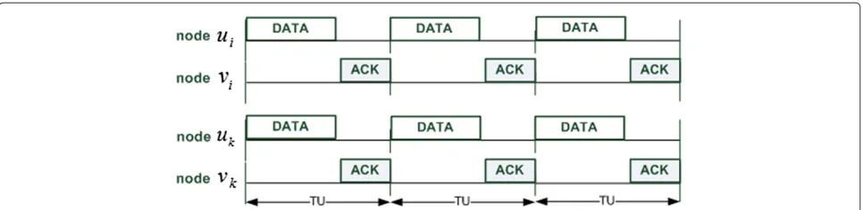
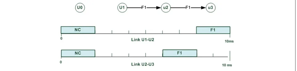
• Starts only at the beginning of a time unit (TU) interval (see Figure 3).
• Lasts the time of a TU (this will be detailed in the next sections, see Equation 6). Note that we assume that all data packets have the same size and thus have the same transmission time.
Hence, no transmitteruj of links(uj,vj) ∈ can send
Figure 3Links(ui,vi)and(uk,vk)transmit simultaneously.The data transmission does not overlap the ack transmission.
(see Figure 3). From the above assumptions and the
SINR-based model, we propose the following interference
model: a transmission on a link(uj,vj)is successful if both
packet data transmission (Equation 4) and acknowledge-ment transmission (Equation 5) are successful:
P d(uj,vj)α
N+
(uk,vk)∈−(uj,vj)
P d(uk,vj)α
≥β (4)
P d(vj−uj)α
N+
(uk,vk)∈−(uj,vj)
P d(vk,uj)α
≥β (5)
When a subsetof links are transmitting simultaneously,
the transmission on the linkei = (uj,vj) ∈ is
success-ful if it respects Equations 4 and 5. LetIbe the distance
matrix of size|V|×|V|. The value of each elementiijofIis
the Euclidean distance between nodeviand nodevj: when
i = j, the value of the elementiijis null, as the Euclidean
distance between a node and itself is null.
3.2 Time division
In our model, we consider that the nodes of our network are synchronized and the time is split in two different intervals (see Figure 4):
• TU interval: a TU interval has a length equal to the time needed for the transmission of a packet. The formula to compute TU’s length is presented hereafter in the paper.
• Transmission scheduling (TS) interval: a TS interval is composed of a fixed numberN of TUs and is periodically repeated everyN×TU.
A TS interval is made up of two periods: the first one is
the period of contention access to the channel denotedTc
and the second is the link scheduling period denotedTs
(see Figure 4). TheTcperiod is made up ofNcTUs (with
Nc < N): during this period, nodes send packets using
CSMA/CA, whereas the TS period is made up ofNsTUs
(withN = Nc+Ns): during this period, nodes transmit
data packets using TDMA.
Scheduling a link consists in selecting the TUs in the
Tsinterval during which the link will be activated without
any risk of interference. In order to give more flexibility in the selection of TUs, the length of a TU must be as short as possible; a TU is equal to the time of a packet transmission, which is the same for all packets:
TU=Tpacket=Tdifs+
L+H
C +Tack+Tsifs+2×TPLCP
(6)
whereLandH, respectively, are the size of a data packet
and its header;TdifsandTsifs, respectively, are the
inter-frame space time of DIFS and SIFS which are defined in
the IEEE 802.11 standard;Tack is the transmission time
of an acknowledgment; andTplcpis the transmission time
of the physical layer convergence protocol (PLCP) header
[4]. The requirements of a flowfare expressed by the
dou-ble f =(brf,drf), where brf represents the minimum
bandwidth required byfanddrf represents the maximum
delay required. The set of flows which are in process are
denotedF. In the sequel, we present and prove two the-orems. These theorems are at the base of our method to compute the delay of any flow knowing its scheduling.
3.3 Link scheduling in terms of bandwidth
For each flow, every nodeuialong its path (except the
des-tination) reserves a fixed number of TUs (denotedTUf) in
the TS interval in order to respect the flow requirements
in terms of bandwidth. For a flowf with a ratebrf,TUf
can be computed with the following formula:
TUf =
where is the ceiling function and TS the length (in
seconds) of a TS interval. The scheduling of a flow
f over a link ei is denoted by a z − tuple, rf(ei) =
(tu(ei)1,. . .,tu(ei)z)wherezis equal toTUf. Each element
tu(ei)jrepresents the position of a TU in the TS interval
during which nodeui such that ei = (ui,vi) must send
a packet of flowf if it possesses any in its queue. These
elements are ordered in ascending order such that:
∀j∈[ 1,TUf −1] and∀ei∈lf,tu(ei)fj <tu(ei)fj+1 (8)
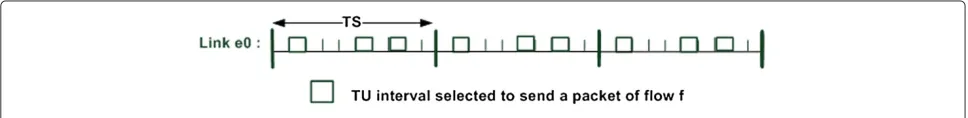
For example, in Figure 5, the schedule of flowf over link
e0isrf(e0)=(2, 6, 8).
3.4 Link scheduling in terms of delay
The link scheduling must respect the delaydrf that every
flowf ∈ F requires. The delay of a flow depends of its
scheduling over every link along its path. A path of a flow
f is denoted aslf = (e0,e1,. . .,en) and must verify the
whereV∗is the set of gateways in the network. In the
fol-lowing, the transmitter nodeuiand the received nodevi
of a link ei possess the same index i as that of the link
it belongs to. Furthermore, this index represents the link
position on the path of a flowf; the index starts at 0. We
denotepfj thejth packet of a flowf. We define the three
following delays:
• Delay of a packet at a link: The delay of a packetpfj at a linkei(withei=(ui,vi)) represents the time between the packet’s arrival at the link’s start nodeui and its correct delivery to the link’s end nodeviand is denoted byd(ei,pfj).
• Delay of a packet: It is the time that takes a packetpfj to cross all links along its path. It is denoted byd(pfj)
and can be computed as follows:
d(pfj)=
∀ei∈lf
d(ei,pfj) (10)
• Delay of a flow: The delay of a flow f is the maximum delay taken by a packet of this flow; it is denoted by d(f). So if a flowf sends n packets, the delay of this flow can be computed as follows:
d(f)=max{S}withS={∀j∈Nand∀j∈[ 0,n−1]|d(pjf)} (11)
The notations used in this section are presented in Table 1.
In the sequel, we fix the starting time (i.e.,t=0) at the
beginning of the TS at which the first packet of flowf is
sent over the linke0. To compute the delay of any flow
f ∈F, we need to introduce the following assumptions:
• The transmitter nodeu0of linke0sends a packet of flowf at each reserved TU for f.
• Nodeu0receives a packet off just before every TU it has reserved forf. Thus, the delay of every packet of f at edgee0is equal to one TU.
• u0sends its first packet at the first TU reserved forf, i.e., at the(tu(e0)1)th TU of the first TS interval,
tu(e0)1∈rf(e0).
• Every nodeuihas a FIFO queue whose length is equal q(ei,t)at timet. The length of every node’s queue is initialized at 0, i.e.,q(ei, 0)=0,∀i∈N.
Lettjbe the time such thattj=TS×j,∀j∈N. Thus, the
timetjis the beginning of the (j+1)th TS interval. In the
following, we introduce two theorems. These theorems are at the base of our method to compute the delay of any flow knowing its scheduling. The first theorem asserts that when a flow enters the network, it becomes stable at a link only after a certain time; once a flow is stable at a link, the start node of the link sends a packet of the flow at every reserved TU and has a queue’s length at the
Table 1 Notations
Notation Description
rf(ei) Represents the set of the reservedTUf TUs during which
linkeihas to send packets of flowf
tu(ei)j Position of thejth TU in the TS interval reserved by linkei
pf
j Thejth packet of the flowf
d(ei,pfj) The delay at the linkeiof the(pfj)th packet sent by flowf
d(pf
j) Delay of the packetpfj tj Timetsuch thatt=TS×j
d(ei)j The delay at linkeiof a packet sent byeiat the(tu(ei)j)th
TU of a TS interval during the stable period ofei
q(ei,t) Length of the nodeui’s queue at timet
beginning of every TS of the same size. The first theorem enables to prove the second theorem. The second theorem asserts that once a flow is stable at a link, the delay of its packets at this link is periodic, of period one TS, i.e., every packet sent at the same reserved TU of any TS interval gets the same delay at this link. Thus, according to the second theorem, the delay of a packet at a link takes only
TUf different values. By computing theseTUf values for
every link, we get the delay of every packet at every link. By adding up the delay a packet gets at every link, we can get the delay of the packet. Then, the delay of the flow is obtained by extracting the highest delay among the delay of every packet of the flow.
3.4.1 Transition and stable periods
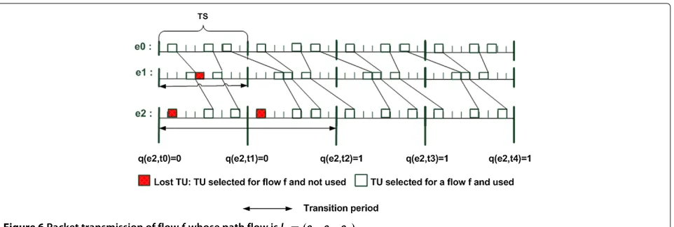
Theorem 1. Before time ti, every link ei(∀ei ∈ lf) is in
a transition period, i.e., its start node ui possesses at the beginning of each TS interval a queue whose length is less or equal to q(ei,ti)(queue’s length of uiat ti) and does not send a packet at each of its reserved TU. From ti, every link ei(∀ei ∈ lf)is in a stable period, i.e., it sends a packet at each of its reserved TU and the length of its queue at the beginning of every TS interval is fixed and equal to q(ei,ti).
We can observe from Figure 6 the transition period of
link e1 which lasts until the end of the first TS interval
and the one of linke2which lasts until the second
inter-val. During link e2’s transition period, we can observe
that its start node does not send a packet at each of its reserved TU. Furthermore, during its stable period, it sends a packet at each reserved TU and possesses at the beginning of every TS interval a queue of length 1.
Proof. Let us prove Theorem 1 by recurrence. First,
Theorem 1 is valid for link e0 as we have previously
assumed thatu0sends a packet at each of its reserved TU
and the delay of any packet of flowf is one TU. Thus, from
t0, nodeu0sends a packet at every reserved TU and has at the beginning of each TS interval a queue of length 0.
Now, let us prove Theorem 1 for every linkei∈lf−{e0}.
At ti−1, ui possesses a queue of length q(ei,ti−1). This queue length is inferior or equal to the one it would
have obtained if ui−1 has sent a packet at each TU it
has reserved since t0. Let us assume that ui−1 has sent
a packet at each reserved TU since t0. During the first
TS interval,uireceivesTUf packets and forwardsz. This
implies that there exist a subset of rf(ei)that we denote
r1f(ei−1) =(tu(ei−1)11,. . .,tu(ei−1)1z)and a subset ofrf(ei)
denotedrf1(ei)=(tu(ei)11,. . .,tu(ei)1z)such that:
∀j∈[ 1,z] ,tu(ei−1)1j <tu(ei)1j (12)
Thus, whenui receives a packet at the(tu(ei−1)1j)th TU,
it can forward it at the(tu(ei)1j)th TU as this TU is
sit-uated after. Thus, at t1, ui possesses a queue of length
TUf −z. During the second TS interval,uifirst sends the
TUf − z packets it possesses in its queue at the
begin-ning of the TSl. Then, it has stillzavailable TUs denoted
r2f(ei) = (tu(ei)21,. . .,tu(ei)2z) and which is a subset of rf(ei). As it is thezlast reserved TU ofui, we get:
∀j∈[ 1,z] ,tu(ei−1)1j <tu(ei)1j <tu(ei)2j (13)
Thus,ui can send a packet at each of itszavailable TUs.
During this second TS,ui sends a packet at each of its
reserved TU and possesses at the end of the TS in its
queueTUf −z packet. As the queue length ofui is the
same att2andt1, it implies that fromt1,uipossesses at the
beginning of each TS intervalTUf−zpackets in its queue.
We can thus conclude that ifui−1had sent a packet at each has in its queue at the beginning of the TS. Thus, it has stillTUf−q(ei,ti−1)TUs available in the current TS
inter-val which can be represented by a subset ofrf(ei)denoted
rf3(ei) = (tu(ei)31,. . .,tu(ei)3TUf−q(ei,ti−1)). As these TUs
are theTUf −q(ei,ti−1)last reserved TUs ofuiand that TUf −q(ei,ti−1)≤z, we getrf3(ei)⊂rf2(ei); then
accord-ing to Equation 13,uican sendzpackets among theTUf
it has received during the TS. Thus, fromti−1toti,uidoes
not send a packet at each reserved TU and linkeiis still in
transition. Atti,uipossessesTUf −zpackets in its queue,
as we have previously seen; once it getsTUf−zTUs at the
beginning of a TS interval,uithen sends a packet at every
reserved TU and possesses a queue of lengthTUf −zat
the beginning of every TS interval. Fromti, linkeigets
sta-ble. Thus, we have proved Theorem 1 by recurrence as it is true for linke0and for any linkei∈lf − {e0}if its previous
linkei−1respects the theorem.
3.4.2 Periodicity of packet delay
Theorem 2. When a link ei becomes stable, the delay
of packets at this link gets periodic, i.e., every packet of flow f that ei’s start node, ui, sends at the reserved TU tu(ei)j(j ∈[ 1,TUf])of any TS has the same delay at the link ei(denoted d(ei)j).
Proof.From Theorem 1, we know that every linkei =
(ui,vi)after timetiis activated at each of its reserved TU
and that ui has a queue of lengthq(ei, ti) at the
begin-ning of each TS interval. Thus, after timeti, when node
ui−1sends a packet at the(tu(ei−1)j)th TU of a TS inter-a bijective function which inter-associinter-ates einter-ach position of inter-a
TU reserved by linkei−1with one reserved by linkeisuch
that whenei−1sends a packet at the(tu(ei−1)j)th TU of
a TS interval situated afterti, link ei forwards it at the
(tu(ei)j)th TU of the current or of the next TS interval
Recall that Theorem 1 asserts that the queue length of a
nodeuiat the beginning of a TS interval in the transition
period is less than (or equal to) that in the stable period.
It implies that whenuireceives a packet during its
transi-tion period, this packet waits less (or the same) time before being sent than during the stable period; the delay for this
packet is at linkei less or equal to the delay in the stable
period. Thus, if we denotepya packet thatuisends during
a stable period at thejth TU andpza packet thatuisends
during a stable period at thejth TU withj∈[ 1,nb(TU)f],
then:
d(ei,pz))≤d(ei,py)andd(ei, py)=d(ei)j (15)
Equations 14 and 15 prove Theorem 2.
3.4.3 Packet and flow delay
Recall that the delay of a packet is the sum of the packet
delay at each link it crosses. Letpybe theyth packet sent
byu0such thaty=z×TUf+jwithj∈[ 1,TUf] andz≥n;
the delay of this packet is:
d(py)=TU+d(e1)j1+d(e2)j2+ · · · +d(en)jn (16)
wherej1is the index of the reserved TU at whiche
1sends
the packetpy(i.e.,tu(e1)j1 = ρe1(tu(e0)j)),j2is the index
of the reserved TU at whiche2sends the packetpy(i.e.,
tu(e2)j2 = ρe1(tu(e1)j1)), etc. Thus, fromtn, there isTUf
different delays for a packet depending at which TU in
the TS intervalu0sends it. The delay of a packet sent at
the(tu(e0)j)th TU of any TS interval (∀j∈[ 1,TUf]) in the
the delay of a flow can be computed with the following
LetSbe the scheduling matrix of size|E|×Nwhich
repre-sents the scheduling made for every flowf ∈F. The value
of each elementsijofSindicates whether theith linkeihas
scheduled a transmission at thejth TU of the TS interval:
sij=
f iftuj∈rf(ei)
0 otherwise (18)
where tuj represents the jth TU of a TS interval. The
matrixSmust satisfy the following constraints:
• The conflict-free constraint: Every link must check the SINR-based model, and so inequalities 4 and 5 and can only be scheduled during TUs of the link scheduling periodTs.
• The bandwidth constraint: For every flowf ∈F, every linkei∈lf (withlf respecting the constraints expressed in 9) must reserveTUf slots forf.
• The flow delay constraint: Every flowf ∈Fmust possess a delay inferior or equal to its requirements.
Each time a new flow f is admitted on the network,
the scheduling matrixSoldmust be updated such that all
the scheduling made for this flow over every linkei ∈ lf
are included to form the new schedule matrixSnew. The
elements ofSneware:
snewij =
soldij ifei∈/lf orj∈/rf(ei)
f ifei∈lf andj∈rf(ei) (19)
At the end of the transmission of f, the scheduleSold is
updated such that all the scheduling made forf over every
linkei∈lf are deleted to form the new scheduling matrix
Snew.
3.6 Problem formulation of the admission control of a flow
As we have explained in the previous section, the
require-ments of a flow f are expressed by f = (brf, drf,).
We therefore propose a method which aims at finding
for every requirement f of a new flow f and a pathlf
the scheduling for every link on the flow path, i.e., to
find rf(ei),∀ei ∈ lf while respecting the three following
constraints:
1. |rf(ei)| =TUf. 2. df ≤drf. 3. Snewis feasible.
For a new flow, if every link on its path can find a schedule for this flow which satisfies these constraints, then the flow is admitted on the network; otherwise, the flow is rejected. Constraint 1 enforces that every link along the path respects the link requirements in terms of band-width. Constraint 2 enforces that the delay of the flow computed via Equation 17 respects the delay required by the new flow. Constraint 3 enforces that the new schedul-ing matrix of the network computed via Equation 19 is feasible, i.e., the scheduling made for previously accepted flows and the new flow are interference free.
4 Admission control
Our proposed admission control scheme is based on the reactive routing protocol AODV; however, packets have been modified in order to meet our approach require-ments. The admission control takes place in three steps:
• Route discovery • Link scheduling • Route selection
4.1 Route discovery
During this phase, a source node broadcasts a route request (RREQ) packet which contains the source sequence number (to uniquely identify each packet), the time-to-live (TTL), the bandwidth, and the delay required by the new flow. Each node which receives the RREQ adds
its identificationidand rebroadcasts it if:
• The TTL has not expired. • The node is not the gateway.
• It is the first time the node receives the RREQ. • It succeeds the partial admission control.
The partial admission control aims at filtering flows’ requests which could not be in the sequel accepted. Every node which receives a RREQ for a flow carries out a partial admission control on the flow; it checks
whether the number of available TUs per Ts is
supe-rior or equal to the numberTUf of TUs required by the
flow. The number TUav of available TUs for a node in
a Ts is equal to the number of TUs during which the
node is neither a transmitter nor a receiver. If TUav ≥
TUf, then the node has enough available bandwidth
to satisfy the flow requirements and thus the partial admission control is achieved; otherwise, the node has not enough available bandwidth and thus the RREQ is dropped.
4.2 Link scheduling
When a RREQ reaches a gateway access point, the lat-ter starts the admission control and the link scheduling process. Note that gateways are the only nodes which
of links can transmit simultaneously without interference. As link scheduling is computed at gateways and as the
latter need the scheduling matrixS up to date to
com-pute valid new link scheduling, thus, gateways have to be kept informed (for instance, via notification exchanges) about when a new flow is scheduled or stopped so that all gateways in the network have the same updated scheduling matrix. Recall that the link scheduling and the admission control are realized simultaneously. Indeed,
a flow f is admitted if scheduling for every link on
the flow path (i.e., ∀ei ∈ lf, rf(ei) exists and satisfies
the constraints cited in Section 3.3). To find a feasible link scheduling, we propose a simple greedy algorithm (Algorithm 1).
Algorithm 1Admission control algorithm based on link
scheduling
which specifies whether thejth TU ofei’s TS interval
is available or not. If a link possesses no available TU, return null.
3: The reservations at every linkei ∈ lf are initiated at
empty, i.e.,rf(ei)=∅.
4: forr=1,r≤TUf,r+ + do
5: UpdateAv(e0)and check if has still available TU(s).
If it has not, return null.
6: Pick randomly one available TU ofAv(e0):av(e0)j.
7: Check ife0can be activated during the(av(e0)j)th
TU according to the SINR-based interference
model. If it is the case, e0 reserves this TU, i.e.,
rf(e0)=av(e0)j; otherwise, return to line 5.
8: fori=1,i≤n,i+ +do
9: Update Av(ei) and check if has still available
TU(s). If it has not, return null.
10: Findav(ei)j the available TU inAv(ei) which is
the closest TU to the one that has just reserved
ei−1and which is situated after it. If there does
not exist any, findav(ei)jinAv(ei)such that it is
the first available TU forei.
11: Check whether link ei can be activated during
the(av(ei)j)th TU such that the resultingSnewis
feasible; if it is the case, linkei reserves it, i.e.,
tu(ei)r=av(ei)j; otherwise, return to line 8
12: end for
13: end for
14: Compute the delaydf of the flow from the source to
the link with Equations 14, 16, and 17. Ifdf > drf,
then return null.
15: Update the scheduling matrix and returnSnew
The algorithm returns null if the flow is rejected; other-wise, it returns a new scheduling matrix (which integrates the link scheduling made for the flow). The algorithm can be divided in three major steps. In a first step, we ini-tiate the parameters used in the algorithm. We compute
TUf, the number of TUs that each link must reserve to
respect the flow constraints in terms of bandwidth (see
Equation 7). We then compute for every linkei ∈ lf its
linear matrix of available TUsAv(ei); each elementav(ei)j
indicates whether thejth TU of the TS interval of linkei
is available (av(ei)j = 0) or not (av(ei)j = 1). An
avail-able TU for a link ei = (ui,vi) is a TU which has not
been reserved by any link possessing either ui or vi or
both as a receiver or a transmitter. In a second step, we
reserve theTUf TUs required by the flow on every link
on the flow path. First, an available TU of linke0(i.e., the
first link on the flow path) is randomly selected via its
lin-ear matrix of available TUsAv(e0). Then, the algorithm
checks ife0can be activated during this selected TU (i.e., if
the resulting scheduling matrix is feasible). If it is the case,
the algorithm reserves fore0this TU; otherwise, it chooses
randomly another possible available TU tille0has no more
available TU inAv(e0)that it has not tested. Once an
avail-able TU has been reserved fore0, we select one available
TU for each upcoming link on the path, such that the selected TU is the closest to the TU that the previous edge has just chosen. The idea is to get the shortest feasible delay for a packet at each link. The algorithm then checks whether the link can be activated during this TU (i.e., if the resulting scheduling matrix is feasible). If it is the case, then the algorithm goes on; otherwise, it chooses another
possible available TU till ei has no more available TU.
Each link on the flow path is processed till every link has reserved one TU. The algorithm uses the same method
to reserve the otherTUf −1 TUs required by the flow at
every link along its path. If it succeeds in scheduling every link, then the algorithm enters its third step. In a third step, the algorithm checks whether the link scheduling that has just been realized respects the flow’s require-ments in terms of delay. First, it computes the start node queue length of every link during its stable period. Then,
it can compute for every linkei ∈ lf − {en}its function
ϕei: rf(ei−1)→rf(ei). Thanks to it and via Equation 14, it
gets the delay of every packet at a link. Then, it computes
theTUf possible delays of any packet in a stable period,
thanks to Equation 16. Finally, by applying Equation 11, it gets the delay of the flow. If the delay of the flow is superior to the required delay, then the algorithm returns null; oth-erwise, it returns the new scheduling matrix and the flow is accepted. This algorithm can be solved in a polynomial time.
to simplify the algorithm. At the beginning, we are in the following situation (see Figure 7): the set of nodes
of the WMN is V = u0,u1,u2,u3 and the set of links
isE = {(e0 = (u0,u1),e1 = (u1,u0),e2=(u1,u2),e3 = (u2,u1),e4=(u2,u3),e5=(u3,u2)}, a flowf1has already been admitted, and the reservations made for this flow are represented in Figure 7. We want to admit a new
flowf2, which required delaydrf2 = 150 ms and required
bandwidth ibrf2 = 100 kbit/s along a path lf2 = (e0 =
(u0,u1),e2=(u1,u2),e4=(u2,u3)). The algorithm takes
in inputC = 1 Mbit/s, TU = 1 ms,TS = 10 ms, P =
15 dBm,β = 20,α = 2,N = −90 dBm,drf2, brf2, lf2,
the distance matrix I, and the scheduling matrix S. The
distance matrix is as follows:
I=
0 100 200 300
100 0 100 200
200 100 0 100
300 200 100 0
where each element iij = d(ui−1,uj−1). The scheduling
matrix is as follows:
S=
Nc Nc 0 0 0 0 0 0 0 0
Nc Nc 0 0 0 0 0 0 0 0
Nc Nc 0 0 0 0 0 0 f1 f1
Nc Nc 0 0 0 0 0 0 0 0
Nc Nc 0 0 0 0 f1 f1 0 0
Nc Nc 0 0 0 0 0 0 0 0
where each element sij represents the jth TU of the
TS interval of the link ei−1. If sij = Nc, the jth TU
of the TS interval is dedicated to control packets. If
sij=0, the link ei−1 does not send any packet at the
jth TU of the TS interval. If sij=fz, the linkei−1 sends
a packet of flow fz during the jth TU of the TS
inter-val. In a first step, the algorithm computes the number of TUs required by this flow per TS using Equation 7,
TUf2 =1. Then, the linear matrix of available TUs of
every link on the flow path is computed: Av(e0) =
(1, 1, 0, 0, 0, 0, 0, 0, 1, 1),Av(e2) = (1, 1, 0, 0, 0, 0, 1, 1, 1, 1), and Av(e4) = (1, 1, 0, 0, 0, 0, 1, 1, 1, 1). The reservations
of every link ei ∈ lf2 are initiated at empty, i.e.,
rf2(ei)=∅.
In a second step, the TUf2 TUs required by the flow
on each link ei ∈ lf2 must be reserved. First, the
algo-rithm checks if there is available TU(s) in the linear matrix
Av(e0). As it is the case, an available TU of the linke0is
randomly picked up, for example, the 7th TU. Then, the
algorithm checks ife0can be activated during the 7th TU
by verifying if the inequalities 4 and 5 are respected. As the inequalities are not respected, another available TU is so
randomly picked up, for example,TU =5. This time, the
inequalities 4 and 5 are respected, and the TU is reserved,
rf2(e1)= (5). Then, the matrix of available TUs of linke2 is updated while considering the reservations that we have previously made; thus, Av(e2) = (1, 1, 0, 0, 1, 0, 1, 1, 1, 1).
The available TU of link e2 which is the closest to the
one reserved by linke0and situated just after it is picked
up; it is the 6th TU. The activation of this TU by linke2
respects the inequalities 4 and 5, and this TU is reserved;
rf2(e2)=(6). Linke4’s linear matrix is updated while
con-sidering the reservations that have been previously made; thus,Av(e4) = (1, 1, 0, 0, 1, 1, 1, 1, 1, 1). As there exists no
available TU of linke4situated after the TU that has just
chosen e2 (the 6th TU), the first available TU of e4 is
picked up, which is the third TU of its TS interval. The inequalities 4 and 5 are respected, and the third TU is
reserved; rf2(e4) = (3). If the flow had required more
TU per TS than one, we would have returned to the sec-ond step in order to reserve for each link another TU. In a third step, we must check if the reservations that have
just been made for flowf2 respect its required delay. As
we have previously made the assumption that the start
node of link e0 receives a packet just before each of its
reserved TUs, the delay of every packet at e2is one TU,
d(e2)1=1TU. We must now compute the delay of every
packet off2at every link on the flow path once every link
is in their stable period. This computation is simplified as every link has reserved one TU per TS; thus, every packet
Figure 8Chain topology.
at a link gets the same delay. Linke2 has a queue at the
beginning of each TS interval of length 0 as its reserved
TU is situated just after that ofe0; thus,ϕe2(5) = 6 and
so according to Equation 14, the delay of the packet at the
linke2,d(e2)1 = 1TU. Linke4has, at the beginning of
each TS interval, one packet in its queue. Indeed, when it receives a packet, it must wait for the next TS interval to
send it; thus,ϕe4(6) = 3 and according to Equation 16,
the packet’s delay at linke4isd(e4)1 = 7TU. Thus, the
delay of any packetpzof flowf2during the stable period
is d(pz) = d(e1)1 +d(e2)1 +d(e4)1 = 1+ 1+ 7 =
9TU. As only one packet is sent by TS, according to
Equation 17,d(f2) = 9 ms. The flowf2is thus accepted
and the algorithm returns the new following matrix:
Snew=
Nc Nc 0 0 f2 0 0 0 0 0
Nc Nc 0 0 0 0 0 0 0 0
Nc Nc 0 0 0 f2 0 0 f1 f1
Nc Nc 0 0 0 0 0 0 0 0
Nc Nc f2 0 0 0 f1 f1 0 0
Nc Nc 0 0 0 0 0 0 0 0
This algorithm is a heuristic approach which aims at solving the problem formulated in Section 4.2. If the flow is not admitted, then the admission control stops;
other-wise, the algorithm returns the new scheduling matrixS
Figure 9Grid topology.
from which the gateway extracts the scheduling for every link of the path. The gateway creates a route response packet (RREP) to which it adds the scheduling for every link on the flow path.
4.3 Route selection
In this step, the gateway unicasts the RREP to the source. The RREP goes through the reverse path of the RREQ. Thus, every node along the path extracts and registers the reservation that the gateway has made for the links it belongs to as either a transmitter or a receiver. Once the RREP reaches the source node, the flow transmission can begin and every node along the path knows at which TUs it must forward the flow. Note that the selected TUs for a link are released if the starting node of the link does not
receive any packet of the flow during a certain periodp.
5 Simulation results
In this section, we conduct a simulation study using ns-2 [31] to evaluate and compare the performance of our pro-posed model, with the DCF MAC IEEE 802.11 standard. We evaluate several performance metrics like throughput, packet loss, and delay, under three different topologies: a chain topology, a grid topology, and a linear topology.
Mesh nodes are distributed in a 1,000 m×1,000 m
cov-erage area. Every mesh node sends video flows to the gateway at a rate of 300 kbit/s and requires an end-to-end
Table 2 Simulation parameters
Layer Parameters Values
Signal propagation Two-ray ground model
Physical layer PLCP preamble 20 μs
Channel capacity 54 Mbit/s
MAC layer TU interval 260 μs
TS interval for the chain topology 30,160 μs
TS interval for the grid topology 29,900 μs
TS interval for the cross topology 30,160 μs
Transport layer UDP size packet 1,000 bytes
delay of 150 ms. The flow identification represents the id of the source node and also its order of arrival in the network. Every node (except the gateway) in the network makes a request to admit a new flow in the network in the order of its source id; thus, node 0 is the first to make a request for a flow, then node 1, etc. Requests are sent periodically at 1 s of interval; node 0 first sends a request for flow 0, and a second after, node 1 makes a request for flow 1, etc. The chain topology is made up of 11 nodes, where the middle node (node 5) represents the gateway (see Figure 8). Thus, ten nodes in the linear topology make a request to admit a new flow. The grid topology is made up of 16 nodes (see Figure 9) and the cross topology is made up of 13 nodes (see Figure 10); node 0 represents the gateway for both topologies. Thus, 15 nodes in the grid network make a request to admit a new flow and 12 nodes in the cross topology.
Note that the length of TS interval is fixed in a way that it accepts many flows; thus, it varies according to the network topology. The different parameters used in simulations are presented in Table 2.
Figures 11, 12, 13, 14, 15 and 16 show the through-put of flows in the different topologies and models. With
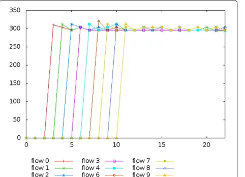
Figure 11Flows’ throughput in our model with a linear topology.
Figure 12Flows’ throughput in the IEEE model with a linear topology.
the linear topology, we can observe in our model (see Figure 11) that among the ten flows which make a request to be admitted in the network, nine flows are accepted and one is rejected. The flow which is rejected is the last to make its request; the network is then too loaded to accept it. The throughput of admitted flows stays quite stable over time, around 300 kbit/s; thus flows’ requirements in terms of bandwidth are respected. In contrary, in the IEEE 802.11 model, the flows’ throughput fluctuates and the 300 kbit/s required is not reached. In the cross topology, we can observe that our model (see Figure 13) accepts 10 flows among the 12 which make a request to be admit-ted. In the grid topology, we can observe that our model (see Figure 15) accepts 10 flows among the 15 which make a request to enter the network. The flows which are not accepted are sent by nodes situated far away from the gateway and which are the last to be sent in the network
Figure 14Flows’ throughput in the IEEE model with a cross topology.
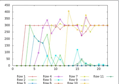
(i.e., flows 10, 12, 13, 14, and 15). As in the linear topol-ogy, our model in the cross and grid topologies meets the flows’ requirements in terms of bandwidth and the flows’ throughput remains quite stable over time, whereas the flows’ throughput in the IEEE 802.11 fluctuates over time and a few of them get their required 300 kbit/s. Figures 17, 18, and 19 show the mean throughput for each flow in the different topologies. Some flows are not indicated on the figures as they are refused by our admission control model and none of their packets reach the gateway in the IEEE 802.11 model. In the chain topology (see Figure 17), all flows which are admitted in the network get the through-put they expected. We can observe that in the DCF IEEE 802.11 model, the more a flow is sent by a node situ-ated far away from the gateway, the more its throughput is low; this phenomenon of starvation is well known and has already been analyzed in many papers (e.g., [32,33]). In the grid topology (see Figure 18), we can observe that in
Figure 15Flows’ throughput in our model with a grid topology.
Figure 16Flows’ throughput in the IEEE model with a grid topology.
the IEEE 802.11 model, as in the previous topologies, the phenomena of starvation for flows are sent by nodes situ-ated more than two hops away from the gateway whereas in our model, every admitted flow gets its required band-width. In the grid topology, as the gateway possesses only two neighboring nodes, only two nodes get almost the required bandwidth of 300 kbit/s (flows 1 and 4). In the cross topology (see Figure 19), as in the previous topolo-gies, IEEE 802.11 suffers from starvation and our model reaches its goal to meet admitted flows’ required band-width. Furthermore, as the gateway in the cross topology possesses only four neighboring nodes, four nodes get almost the required bandwidth of 300 kbit/s (flows 1, 4, 7, and 10). Our link scheduling scheme respects the throughput requirement for flows which are accepted in the network and shows an important gain compared to IEEE 802.11. This gain in throughput can be explained by many reasons such as:
Figure 18Throughput of the flows in the grid topology.
• The elimination of the RTS/CTS scheme. Indeed, as there is no risk of contention, the RTS/CTS scheme is not needed any more. Thus, the time used to send RTS or CTS packet in the IEEE 802.11 model can be exploited to send packets of data in our model. • The elimination of the backoff procedure during the
scheduling period. Indeed, because of the backoff algorithm in the IEEE 802.11 model, every node must wait a certain time, each time it wants to send a packet of data. The time that a node has to wait is chosen randomly in a contention window. The maximum contention window size is 1,023 slots [34] and a slot time lasts usually 20 μs; thus, a node can have to wait till 2,046 μs for sending a packet whereas sending a packet takes, in our example, 260 μs. Thus, eliminating the backoff procedure enables gaining a lot of time for sending packets of data.
Figure 19Throughput of the flows in the cross topology.
Figure 20Packet loss ratio in a chain topology.
• No risk of collision, thanks to the link scheduling. Because of collisions, in the IEEE 802.11 model, nodes need to resend packets; this leads to a waste of time which is avoided in our model.
Figures 20, 21, and 22 show the packet loss ratio of flows in the three different topologies. We can observe that our dynamic link scheduling reaches its goal of collision-free transmission for admitted flows. However, these results are obtained in an ideal state of simulation; indeed, packet loss may occur in a real environment. In IEEE 802.11, we can observe that the more the source of flow is situated far away from the gateway, the more the flow has a high packet loss ratio.
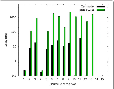
Figures 23, 24, and 25 show the flows’ delay in the
dif-ferent topologies. TheYaxis of these graphics possesses a
logarithmic scale as the values of the flows’ delay are very scattered. We observe in the grid topology (see Figure 24) that flows 10, 12, 13, 14, and 15 in our model possess no
Figure 22Packet loss ratio in a cross topology.
delay as these flows are not admitted in the network, and flows 14 and 15 in IEEE 802.11 possess no delay as none of their packets reach the gateway. For all these topologies, we can observe that our model satisfies the requirements of all flows in terms of delay as they get a delay infe-rior to 150 ms. For all the topologies, the IEEE 802.11 model expresses a delay inferior to 150 ms when their flow sources are situated at less than two hops away from the gateway; for the other flows, the obtained delay is superior to 150 ms.
Through these simulations, we can conclude that our dynamic link scheduling-based admission control model allows gaining in throughput, thanks to the dynamic time division multiple access (DTDMA) access method which enables getting rid of the backoff and RTS/CTS mechanisms. Furthermore, the delay and loss rate require-ments are also satisfied compared to the IEEE 802.11 model. However, in our model, constraints are imposed, nodes must be synchronized, and gateways must know the
Figure 23Flows’ delay in the chain topology.
Figure 24Flows’ delay in the grid topology.
power of the noise and the path loss of the signal at every moment.
6 Conclusion
In this paper, we have presented a new admission con-trol scheme based on link scheduling to support real-time traffic in WMNs. We have considered both bandwidth and end-to-end delay as two major criteria in the design. The link scheduling is based on the SINR interference model in order to prevent any collision in flow packets. To enable a dynamic link scheduling, we have mixed two access methods: on one hand, CSMA/CA is used to send control packets (e.g., requests for flow admission) and on the other hand, DTDMA exploited for flow packet trans-mission, ensuring an important gain in throughput and a collision-free communication. Furthermore, we have introduced a method to compute the flow’s delay and prove its efficiency. We have compared our model with the IEEE 802.11 model and shown under different topologies