Review of Graph Based Scheduling Algorithms
Gagandeep Singh
1, Gurjyot Kaur
2, Dr.Gurvinder Singh
31 2
Research Scholar, Department of Computer Science, Guru Nanak Dev University, Amritsar
3
Head of Department, Department of Computer Science,, Guru Nanak Dev University, Amritsar
Abstract
:For the problem of task scheduling in a parallel program the weighted directed acyclic graphDAG) is used with a set of homogenous processors for the completion of program in the minimized time.There has been a great demand for high speed computing in many application areas. High speed electronic devices were developing to achieve high computing speed. But, the processing speed of uniprocessor computer can’t be increased beyond a limit (few million floating point operations per second) because of the physical limitations imposed by the electrical properties of electronics devices [1]. To achieve high performance, major developments and improvements in the field of processing techniques and computer architectures have been made. Thus, parallel processing approach had gradually emerged to meet the computational requirement of various problem and also to enhance the efficiency of solving various current applications like weather forecasting, military defense, medical diagnosis, simulation, etc.There are many researchers have proposed so many algorithms for scheduling problems, most of these are reported to be efficient, but it is not clear how they compare against each other. Due to many number of issues, it is difficult to measure the actual performance of algorithms and then comparison of these algorithms is also a difficult task.First, most of the scheduling algorithms are based upon diverse assumptions,
making the performance comparison rather
purposeless. Second, standard set of benchmarks to examine these algorithms is not available due to which the actual performance evaluation is not possible. Third, small problem sizescannot evaluate the actual performance of algorithms. The main purpose of this paper is to provide the taxonomy for classifying various algorithms of different categories according to their assumptions and functionalities.
In this paper we discussed 14 scheduling algorithms
and give the characteristics of all algorithms.
Keywords:
Multiprocessors,
parallel
processing,scheduling, task graphs, scalability.
1.
INTRODUCTION
The problem of scheduling a DAG, also called a taskgraph or macro-dataflow graph.In the DAG a set of nodes is used. The set of nodes are homogeneous processors , are used for scheduling the tasks for execution the minimized time [11]. The scheduling problem is NPcomplete in its general forms [9], and only for a fewrestricted cases the polynomial time solutions are available[4], [8]. It is difficult to scheduling the problemin an efficient manner for achieving a meaningful speedup in a parallel or distributed system, so it is important to make the interest of researchers ofall research community to make the efficient execution algorithms. Considerable research effortsexpended in solving the problem by using many heuristic algorithms. While eachheuristic is individually reported to be efficient, it is not clear how these algorithms compareagainst each other on a unified basis.
The objectives of this study include the 14 different algorithms under the categories of UNC, BNP, APN and their characteristics. In this literature survey the large number of DSAs have been presented with different assumptions, it is important to define thesealgorithms into various classes according to their assumptions about the program andmachine model. After its execution, it generates its outputs. In this model,
a set of v nodes {n1,n2,……,nn} are connected by a set of e
directed edges, each of which is denoted by (ni, nj), where
n, is called the parent and nj is called the child. A node
without parent is called an entry node and a node without child is called an exit node. The weight of a node, denoted
by w (ni) , is equal to the process execution time. Since
(ni, nj) is equal to message transmission time. Thus, c (ni,
nj) becomes zero when n, and n, are scheduled to the
same processor communication time[2].
Fig.1 Directed acyclic graph
Consider above directed acyclic task graph G = {V,E} of n
nodes. Each node V = {T1,T2,……, Tn} in the graph
represents a task. Aim is to map every task to a set P =
{P1,P2, . . . ., Pm} of m processor. Each task Ti has a weight Wi
associated with it, which is the amount of time the task takes to execute on any one of the m homogeneous
processors. Each directed edge eij indicates dependence
between the two tasks Ti and Tjthat it connects. If there is a
path from node Ti to node Tjin the graph G, then Ti is the
predecessor of Tj and Tj is the successor of Ti. The
successor task cannot be executed before all its predecessors have been executed and their results are available at the processor at which the successor is scheduled to execute. A task is “ready” to execute on a processor if all of its predecessors have completed execution and their results are available at the processor on which the task is scheduled to execute. If the next o be executed on a processer is not yet ready, the processor remains idle until the task is ready. The elements set C are
the weights of the edges s C = {ck: k = 1, 2, 3 ….r}
Itrepresents the data communication between the two tasks, If they are scheduled to different processors. But if both tasks are schedule to the same processor, then the weight associated to the edge becomes null[13].
If the node nischeduled on the processor P then the start
time and the finish time of node ni is denoted by ST(ni, P)
and FT(ni, P) respectively.The main objective of the DAG
scheduling is to find the earlier start time of the tasks to the processors such that schedule length minimized such that the precedence constraints are preserved.
For solving the problem of DAG scheduling mostly the researchers are interested to design efficient heuristics which can find the better solution for the problem within a reasonable amount of time. Most of these heuristic
algorithms are based on the list scheduling techniques.
The concept of priority assignment is used. The priorities are assigned to the nodes and nodes are arranged in descending order of priorities. Higher priority node is scheduled before lower priority node.
Assigning Priorities to Nodes: The t-level(top level) and
b-level (bottom b-level) are the two major attributes which are
used to assigning priorities. The t-level of a node ni is the
length of the longest pathfrom an entry node nito in the
DAG (excludingni ). Here, the length of a path is the sum of
allthe node and edge weights along the path. The t-level of
nihighly correlates with ni’s earlieststart time, denoted by TS(ni), which is determined afterni is scheduled to a processor.
Fig.2 (a)The Static Levels (SLs) t-levels, b-levels and ALAP
The b-level of a node is the length of the longest path from node to an exit node and is bounded by the length of the critical path. The path from an entry node to an exit node, whose length is the maximum is called critical path (CP) of a DAG.
In the b-level of a node variations in the computations are
possible. Most DSAs examine anode for scheduling only after all the parents of the node have been scheduled. In
this case, theb-level of a node is a constant until after it is
scheduled to a processor. However, somealgorithms allow the scheduling of a child before its parents. In that case, the b-level of a nodebecomes a dynamic attribute. Different
DSAs have used the t-level and b-level attributes in a
variety of ways. Some algorithms assign a higher priority to a node with a larger b-level while some algorithmsassign a higher priority to a node with a smaller t-level.
Critical-Path-Based vs. Non-Critical-Path-Based:
Critical-path-based algorithmsgive a higher priority to a
critical-path node (CPN). Noncritical-path-based
algorithmssimply assign priorities based on the levels of the nodes.
Static List vs. Dynamic List: The ready list maintained a
set of ready nodes. The ready list is sorted in descending order. Initially, only the entry nodes are included in the ready list. After a node is scheduled,the next node which is not scheduled is inserted into the ready list.
The list can be maintained in two ways: static readylist and dynamic ready list. In the static ready list the list is constructed before scheduling starts and remains the same throughout the wholescheduling process and in the dynamic ready list the list is rearranged according to the changing node priorities.
Greedy vs. Non-Greedy: Most scheduling
algorithmsattempt to minimize the start-time of a node for assigning a node to a processor. This is a greedy strategy. But in Non greedy, thealgorithms do not minimize the start-time of a node but consider other factors as well.
Time-Complexity: The some termslikenumber of node, the
number of edges, and the number of processorsare used to calculate the time-complexity of a DSA.The main stepof algorithm is to traverse the DAG and search of slots in the processors to place anode. The dynamic priority assignment having higher time-complexity as compared to static priority assignment.
2.
LITERATURE SURVEY
(Adam et al, 1974) discussed the comparison of list
scheduling algorithms for the parallel processingsystem. This paper describe that how list scheduling algorithms vary their performance in the different situations in the parallel environment.
(Ahmed et al, 1997) is describe the concept of automatic
parallelization an scheduling of programs on
multiprocessor environment using CASCH.
(Grahmet al, 1972) is discussed the optimal ways of scheduling of tasks on Two-Processor system.
(Loiet al, 1995) is discussed the techniques of automatic graph generation for scheduling the tasks on the processors in the efficient manner so that the total time of execution can be minimized.
(Lewis et al, 1990) this paper discussed the concept of
scheduling of parallel programs on the arbitrary number of
machines. This paper also gives the comparison analysis of the performance of the scheduling when the number of processors arenon uniform.
(Fernadezet al, 1973) discussed the concept of BNP scheduling. It also describes time for multiprocessors optimal schedule for the bounded number of processors.
(Hwang et al, 1989) discussed the Scheduling of the
precedence graph having the inter-processor
communication time in the multiprocessor environment.
(Kim et al, 1988) This paper describes the General
approach to mapping of parallel computation upon multiprocessor architectures.
(Gurvinder Singh et al, 2011) It is the survey paper about all the scheduling algorithms that allocates parallel program to DAG on homogenous processors. The main suboptimal solutions in less than the polynomial time.
3.
TAXONOMY
OF
DAG
SCHEDULING
computational costs. The earlier work done by researchers the inter-task communication assumed to be zero, that is, the task graph contains precedence but without cost. The problem becomes less complex in the absence of communication delays.For minimizing the communication delays of scheduling the task duplication is used.Duplication is done by duplicating the ancestor nodes on which the predecessors of those nodes are dependent for the execution.
There are two former classes of algorithms of list scheduling problems are called the UNC i.eunbounded number of clustersscheduling algorithms [2] and the BNP i.ebounded number of processors scheduling algorithms [2]. In both classes of algorithms, the processors are assumed
3.1.UNC Scheduling Algorithm
The concept of clustering is used in UNC algorithms. Each node in UNC considered as a cluster. In this algorithm the merging of the clusters is done if it reduces the completion time. Merging continuously performed until no cluster can be merged. The idea behind UNC algorithm is that it uses more processors to further reducing the schedule length. The post processing step is performed for mapping the clusters onto the processors because the cluster may be more than the number of processors.
In UNC scheduling we have study the five algorithms named as EZ, LC, DSC, MD, DCP and study their characteristics.
The EZ Algorithm: This Edge Zeroing algorithm [15] based on edge weights clusters are selected and then merging those clusters. The algorithm finds the edge with the largest weight at each step. Thetwo clusters incident by the edge are merged and the mergingis done if and only if it does not increase the completion time. After merging the two clusters, the SLs of the nodes are used for ordering of the nodes in the resultant cluster.
The LC Algorithm: This Linear Clustering algorithm [13] forming asingle cluster based on the CP by merging the nodes. In the first step the set of nodes constituting theCP is determined by the algorithm. Then it schedules all of the CP nodes to a single processor at once. The scheduled nodes and all incidentedges are then removed from the DAG. The algorithm zeroes the edges onthe entire CP at once.
The CP may change when an edge is zeroed. The original CP is not containing the edge that should be zeroed next.
The DSC Algorithm: The Dominant Sequence Clustering algorithm [9] considersthe Dominant Sequence of a graph. It is simply the CP of the partially scheduledDAG. The DSC algorithm tracks the CP of the partially scheduled DAG at
each step. For this it uses the composite attribute (b-level + t-level) as the priority of a node. Unless the node is ready, the DSC algorithm does notselect the node having the highest priority for scheduling.
The MD Algorithm:If a node is on the current CP of the
partially scheduled DAG, the sum of its b-level and t-levelis
equal to the current CP length. Thus, the relative mobility of a node is zero if it is on thecurrent CP. At each step, the MD algorithm selects the node with the smallest relative mobilityfor scheduling. In testing whether a cluster can accommodate a node, the MD algorithm scansfrom the earliest idle time slot on the cluster and schedules the node into the first idle time slotthat is large enough for the node.
The DCP Algorithm: The Dynamic Critical Path algorithm [14] is designed basedon asimilar attribute to relative mobility. To find a better
cluster this algorithm uses a look-ahead strategy
for a given node. In addition, The DCP algorithm
computes the value of TS(nc) on a cluster for computing the
value of TS(n1) on the same cluster, where,ncis the child of
ni has the largest communication and is called the critical
child of ni. TheDCP algorithm schedules nito the cluster
that gives the minimum value of the sum of thesetwo attributes. This look-ahead strategy can potentially avoid scheduling a node to a cluster
that has no room to accommodate a heavily communicated child of the node. The DCP algorithm examines all the existing clusters for a node while the MD algorithm only tests fromthe first cluster and stops after finding one that has a large enough idle time slot.
Algorithm Priority List CP Based Greedy Complexity
Table 1: UNC Scheduling Algorithm and their characteristics
3.2.BNP Scheduling Algorithms[3]
In this scheduling technique we have discussed five algorithms: HLET, MCP, ISH, ETF, LAST. The characteristics
are given in the table below where p denotes the number of processors given.
The main drawback of HLFET is that itcalculating the SL of a node and ignores the communication costs on the edges.
The ISH Algorithm: The ISH i.e Insertion Scheduling Heuristic algorithm [14] uses the holes created by the partial schedules with simple but effective idea. It first picks anunscheduled node. The processor that allows the earlieststart time is used to schedule the unscheduled node having highest SL. It tries to insert other unscheduled nodes from the ready list into the idle time slotbefore the node just scheduled.
The MCP Algorithm: The MCP i.e Modified Critical Path algorithm [16] uses the ALAPtime of a node as a priority. For computing the ALAP time
of a node, first computing thelength of CP and then
subtracting the b-level of the node from it. Thus, t-level on
the CP are the ALAP times of the nodes. After computing the ALAP times of allthe nodes, MCP algorithmthen constructs a list in ascending order of ALAP times of all the nodes.
Ties arebroken by considering the ALAP times of the children of a node. Thenone by one the algorithm schedulesthe nodes on the list such that the insertion approach is used for scheduling and the processor that allows theearliest start time is used for scheduling a node.
The ETF Algorithm: The ETF i.e Earliest Time First algorithm [10] selects the node having smallest start time. For finding smallest start time firstly earliest start time of all the nodes are computed at each step.The tie of two nodes having same earliest start time breaks by scheduling the one with the higher SL. Thus, a node with ahigher SL does not necessarily get scheduled first because node with the earliest start time having higher priority according to the algorithm.
The LAST Algorithm: The LAST i.eLocalized Allocation of Static Tasks algorithm [9] is nota list
scheduling algorithm. It uses an attribute called D_NODE for the node priority. It depends on the incident edges of a node. The main Objective of this algorithm is to reduce the overall communication. In this algorithm the node can be selected before its parent for scheduling.One of the consequences of using D_NODE is that anode may be selected before some of its parents for the scheduling. Thus, until the scheduling process terminates the earliest start time ofa node cannot be fixed. For the node selection process the node weight is ignored in the LAST algorithm.
Algorithms Priority CP-Based List Type Greedy Complexity
HLEFT SL No Static Yes O(v2)
ISH SL No Static Yes O(v2)
MCP ALAP Yes Static Yes O(v2 logv)
ETF SL No Static Yes O(pv3)
LAST Edge weights No Dynamic Yes O(v(v + e))
Table 2: BNP Scheduling Algorithm and their characteristics
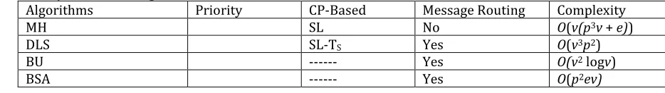
3.3.APN Scheduling Algorithms
APN Scheduling we have discussed four algorithms MH, DLS, BU, BSA and the characteristics are given in the below table.
The MH Algorithm: The MH i.eMapping Heuristic algorithm [7] initially makes a ready nodelist. It contains entries of all nodes arranged in descending orderaccording to their priorities. Theprocessor having the smallest start time is used for scheduling the node. A routingtable is used in this algorithm which maintained the calculated start timeof a node for each processor. The table contains theinformation from the parent nodes to the nodes underconsideration. When a node isscheduled on processor all of its ready successor nodes are appended to the ready node list.
The DLS Algorithm: The DLS i.e Dynamic Level Scheduling algorithm [11] is used as an APN scheduling algorithm. In the APN schedulingalgorithm,The message routing method are required for DLS. These routing methods are supplied by the user. Then based on that how
the message is routed from the parents of the node, the TS
of a node is computed
communication messages among all the nodes assigned to processors using a channel allocation heuristic to keep the hop count of every message. Different networktopologies require different channel allocation heuristics.
The BSA Algorithm: The BSAi.eBubble Scheduling and Allocation algorithmconstructs a schedule incrementally. For this it first injecting all the nodes to the pivot processor,defined as the processor with the highest degree. Then algorithm tries to improve the starttime of each node by transferring it to one of the
adjacentprocessor of the pivot processor if the migration can improve the start time of the node. This isbecause after a node migrates, the space it occupies on the pivot processor is released and can be used for its successor nodes on the pivot processor. After all
nodes on the pivot processorare considered, the algorithm selects the next processor in the processor list to be the new pivotprocessor. The process is repeated by changing the pivot processor in a breadth-first order.
Algorithms Priority CP-Based Message Routing Complexity
MH SL No O(v(p3v + e))
DLS SL-TS Yes O(v3p2)
BU --- Yes O(v2 logv)
BSA --- Yes O(p2ev)
Table 3: APN Scheduling Algorithm and their characteristics
4.
CONCLUSIONS AND FUTURE WORK
In this paper we have studied 14 different algorithms for the DAG scheduling problems and their characteristics are discussed. After this we have concluded that:
As demonstrated by both DCP and DSC algorithm
APN algorithm is complicated because it take uses more parameters.
In UNC algorithms the bounded numbers of
processors are used to assigning the clusters obtained through scheduling and all nodes of cluster assigned to a same processor. Due to this property cluster scheduling algorithms become more complex as compared to BNP scheduling algorithms.
BNP and UNC classes’ algorithms having more
accurate performance than other scheduling algorithms.
In the future work these algorithms can be implemented using the Genetic Approach (GA). The Genetic algorithms (Gas) are adaptive heuristic search based algorithms based on the evolutionary idea of natural selection and genetics. GAs are a part of evolutionary computing, a rapid growing area of artificial intelligence. The scheduling algorithms with Genetic Approach give better performance than the simple scheduling algorithms.
5.
REFERENCES
[1] T.L. Adam, K.M. Chandy, and J. Dickson, “A Comparison
of List Scheduling for ParallelProcessing Systems,” Comm.
ACM, vol. 17, no. 12, pp. 685-690, Dec. 1974.
[2] I. Ahmad, Y.-K. Kwok, M.-Y.Wu, and W. Shu, “Automatic
Parallelization and Scheduling ofPrograms on
Multiprocessors using CASCH,” Proc.
1997 Int’l Conf. Parallel Processing, pp. 288-291,Aug. 1997. [3] ParneetKaur, Dheerendra Singh, Gurvinder Singh and Navneet Singh3,“Analysis, comparison and performance evaluation of BNP schedulingalgorithms in parallel processing” , International Journal of Information Technology and Knowledge ManagementJanuary-June 2011, Volume 4, No. 1, pp. 279-284,
[4] Sachi Gupta, GauravAgarwal, and Vikas Kumar, “An Efficient and Robust Genetic Algorithm for Multiprocessor Task Scheduling” , International Journal of Computer Theory and Engineering, Vol. 5, No. 2, April 2013.
[5] E.G. Coffman and R.L. Graham, “Optimal Scheduling for Two-Processor Systems,” Acta
Informatica, vol. 1, pp. 200-213, 1972.
[6] M. Cosnard and M. Loi, “Automatic Task Graph
Generation Techniques,” Parallel ProcessingLetters, vol. 5,
no. 4, pp. 527-538, Dec. 1995.
[7] H. El-Rewini and T.G. Lewis, “Scheduling Parallel
Programs onto Arbitrary Target Machines,” J.Parallel and
Distributed Computing, vol. 9, no. 2, pp. 138-153, June 1990.
[8] E.B. Fernadez and B. Bussell, “Bounds on the Number of
Processors and Time for MultiprocessorOptimal
Schedules,” IEEE Trans. Computers, vol. C-22, no. 8, pp.
[9] M.R. Garey and D.S. Johnson, Computers and Intractability: A Guide to the Theory of NP-Completeness,W.H. Freeman and Company, 1979.
[10] J.J. Hwang, Y.C. Chow, F.D. Anger, and C.Y. Lee,
“Scheduling Precedence Graphs in Systems
withInterprocessor Communication Times,” SIAM J.
Computing, vol. 18, no. 2, pp. 244-257, Apr. 1989.
[11] K. Hwang and Z. Xu, Scalable Parallel Computing:
Technology, Architecture, Programming, McGraw-Hill, 1998.
[12] Y.C. Chung and S. Ranka, “Application and Performance Analysis of a Compile-Time
Optimization Approach for List Scheduling Algorithms on
Distributed-MemoryMultiprocessors,” Proc.
Supercomputing’92, pp. 512-521, Nov. 1992.
[13] S.J. Kim and J.C. Browne, “A General Approach to Mapping of Parallel Computation upon
Multiprocessor Architectures,” Proc. 1988 Int’l Conference
on Parallel Processing, vol. II, pp. 1-8, Aug.1988.
[14] B. Kruatrachue and T.G. Lewis, “Duplication Scheduling Heuristics (DSH): A New PrecedenceTask Scheduler for Parallel Processor Systems,” Technical Report, Oregon State University,Corvallis, OR 97331, 1987.
[15] V. Sarkar, Partitioning and Scheduling Parallel
Programs for Multiprocessors, MIT Press, Cambridge,MA, 1989.