A new chaotic behavior of a general model of the Henon map

R E S E A R C H

Open Access

A new chaotic behavior of a general model of

the Henon map

Ahmed MA El-Sayed

_{, Zaki FE El-Raheem}

_{and Sanaa M Salman}

*_{Correspondence:} [email protected] 1_{Department of Mathematics,}

Faculty of Science, Alexandria University, Alexandria, Egypt Full list of author information is available at the end of the article

Abstract

In this paper we are concerned with a general form of the Henon map as a retarded functional equation. The existence of a unique solution is proved. The continuous dependence of the solution and the local stability of fixed points are investigated. Chaos, bifurcation and chaotic attractor of the resulting system are discussed. In addition, we compare our results with the discrete dynamical system of the Henon map.

Keywords: retarded functional equation; Henon map; fixed points; existence; uniqueness; bifurcation; chaos; chaotic attractor

1 Introduction

Discontinuous (sectionally continuous) dynamical systems have been defined as a prob-lem of retarded functional equation and studied in [–]. The generalized time-delayed Henon map was introduced in [, ]. In this work we study the discontinuous (section-ally continuous) dynamical system of the Henon map as a problem of retarded functional equation with two different delays

x(t) =  +βx(t–r) –αx(t–r), r,r> ,t∈(,T], (.)

with

x(t) =x, t≤, (.)

whereα>  and|β|< .

The existence of a unique continuous dependence solution is proved. The local stabil-ity of fixed points is studied. The chaos, bifurcation and chaotic attractor are discussed. Comparison with the corresponding discrete dynamical system of the Henon map

xn+=  +βxn––αxn, n= , , , , . . . , (.)

is given.

Letf : [,T]×Rn_→Randr

,r, . . . ,rk∈R+.

Consider the problem of retarded functional equation

x(t) =fx(t–r),x(t–r), . . . ,x(t–rk)

, t∈(,T], (.)

with the initial condition

x(τ) =φ(τ), τ≤. (.)

IfT is a positive integer,rk=k,φ() =x, andt=n= , , , . . . , then problem (.)-(.)

will be the discrete dynamical system

xn=f(xn–,xn–, . . . ,xn–k), n= , , , . . . ,T, (.)

x() =x. (.)

This shows that discrete dynamical system (.)-(.) is a special case of the problem of retarded functional equation (.)-(.).

Consider also the singularly perturbed differential difference equation []

x(t) = –x(t) +fx(t– ), (.)

and the singularly perturbed delay differential equation []

x(t) =ax(t) +

The limiting cases as → of (.) and (.) are special cases of retarded functional equation (.)-(.).

Repeating the process we can easily deduce the solution of (.)-(.) which is given by

x(t) =xn(t) =fn

which implies that the solution of problem (.)-(.) is discontinuous (sectionally contin-uous) on (,T].

Now we have the following definitions.

Definition  The fixed points of discontinuous (sectionally continuous) dynamical sys-tem (.)-(.) are the solution of the equation

x(t) =f(t,x,x, . . . ,x). (.)

Remark  We should notice that the difference equations representing the Henon map in its different cases,

xn+=  +βxn––αxn–, n= , , , , . . . ,

xn+=  +βxn–αxn–, n= , , , , . . . ,

xn+=  +βxn–αxn, n= , , , , . . . ,

are just special cases of our problem (.)-(.).

2 Existence and uniqueness

Now consider the discontinuous (sectionally continuous) dynamical system of the Henon map (.)-(.). The existence of a unique solution as well as the continuous dependence of the solution on the initial data are proved. We study also the continuous dependence of the solution on the parameterα.

LetL=L[,T],T<∞, be the class of Lebesgue integrable functions on [,T] with the

Definition  By a solution of problem (.)-(.) we mean that the functionx∈L_satisfies

problem (.)-(.).

Thus we can get

Fx–Fy ≤ |β| x–y + αk x–y . IfM=|β|+ αk< , then

Fx–Fy ≤M x–y .

So, problem (.)-(.) has, onD, a unique solutionx∈L_. Continuous dependence on the initial conditions

Theorem  The solution of discontinuous(sectionally continuous)dynamical system(.) -(.)is continuously dependent on the initial data.

Proof Letx(t) andx∗(t) be the solutions of dynamical system (.)-(.) and the dynamical system of equation (.) with the initial data

x() =x∗_. (.)

Continuous dependence on the parameter

α

Theorem  The solution of discontinuous(sectionally continuous)dynamical system(.) -(.)is continuously dependent on the parameterα.

Proof Letx(t) andx∗(t) be the solutions of dynamical system (.)-(.) and the dynamical system

x(t) =  +βx(t–r) –α∗x(t–r), (.)

with the initial data (.), then

which gives

Exactly like its discrete counter part, dynamical system (.)-(.) has two fixed points which are the solutions of the equation

x=  +βx–αx.

point, consider a small perturbation from the fixed point by letting

x(t) =xfix+λt.

which implies that the fixed points are asymptotically stable if all roots of the equation

 =βλ–r_{– αx}

In all the simulations,randrare rationally dependent.

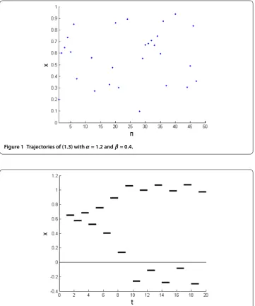
Figure 1 Trajectories of (1.3) withα= 1.2 andβ= 0.4.

Figure 2 Trajectories of (1.1) withα= 1.2,β= 0.4, andr1=r2= 1.

4 Bifurcation and chaos

In this section we show, by numerical experiments illustrated by bifurcation diagrams, that the dynamical behavior of discontinuous (sectionally continuous) dynamical system (.)-(.) is completely affected by the change in both randT []. We consider three cases for different delaysrandras follows.

•Case :r>r.

Letβ= . be fixed and varyαfrom  to . with step size . and the initial condition (x,y) = (., ).

Taker=  andr=  andt∈[, ] in (.)-(.) (Figure ).

Taker= . andr= . andt∈[, ] in (.)-(.) (Figure ).

Taker= . andr= . andt∈[, ] in (.)-(.) (Figure ).

Figure 3 Bifurcation of (1.1)-(1.2) whenr1= 2 andr2= 1 andt∈[0, 150].

Figure 4 Bifurcation of (1.1)-(1.2) whenr1= 0.50 andr2= 0.25 andt∈[0, 38].

Figure 5 Bifurcation of (1.1)-(1.2) whenr1= 0.3 andr2= 0.1 andt∈[0, 20].

We see clearly in Figure  the bifurcation from a stable fixed point to a stable orbit of period two atα= ., and then the bifurcation from period two to period four atα= .. The further period doubling occurs at decreasing increments inα, and the orbit becomes chaotic forα..

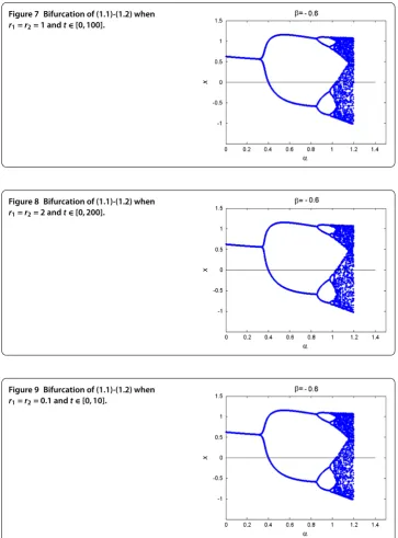
•Case :r=r.

Taker=r=  andt∈[, ] in (.)-(.) (Figure ).

Taker=r=  andt∈[, ] in (.)-(.) (Figure ).

Taker=r= . andt∈[, ] in (.)-(.) (Figure ).

Taker=r= . andt∈[, ] in (.)-(.) (Figure ).

Figure 7 Bifurcation of (1.1)-(1.2) when r1=r2= 1 andt∈[0, 100].

Figure 8 Bifurcation of (1.1)-(1.2) when r1=r2= 2 andt∈[0, 200].

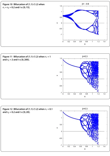
Figure 10 Bifurcation of (1.1)-(1.2) when r1=r2= 0.2 andt∈[0, 15].

Figure 11 Bifurcation of (1.1)-(1.2) whenr1= 1 andr2= 2 andt∈[0, 200].

Figure 12 Bifurcation of (1.1)-(1.2) whenr1= 0.1 andr2= 0.2 andt∈[0, 20].

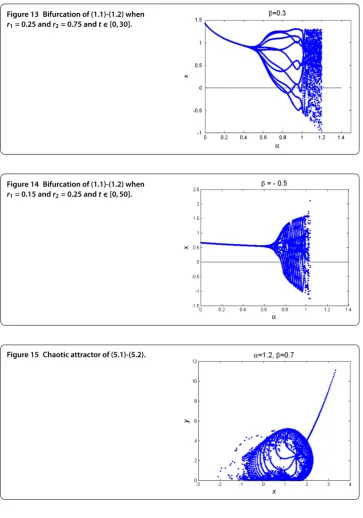
•Case :r<r.

Taker=  andr=  andt∈[, ] in (.)-(.) (Figure ).

Taker= . andr= . andt∈[, ] in (.)-(.) (Figure ).

Taker= . andr= . andt∈[, ] in (.)-(.) (Figure ).

Taker= . andr= . andt∈[, ] in (.)-(.) (Figure ).

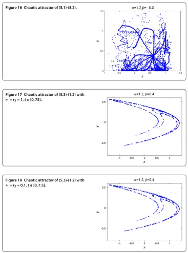
5 Chaotic attractor

In this section we are interested in studying the chaotic attractor for three different cases.

Figure 13 Bifurcation of (1.1)-(1.2) when r1= 0.25 andr2= 0.75 andt∈[0, 30].

Figure 14 Bifurcation of (1.1)-(1.2) when r1= 0.15 andr2= 0.25 andt∈[0, 50].

Figure 15 Chaotic attractor of (5.1)-(5.2).

Here we rewrite system (.)-(.) as follows:

x(t) =  +βx(t–r) –αy(t–r), (.)

y(t) =xt– (r–r)

. (.)

It is worth here to mention what we get when we plot the chaotic attractor for system (.)-(.) in this case. Figure  shows the chaotic attractor whenr=  andr= , while

Figure  shows the chaotic attractor of the same whenr= . andr= ..

Figure 16 Chaotic attractor of (5.1)-(5.2).

Figure 17 Chaotic attractor of (5.3)-(1.2) with r1=r2= 1,t∈[0, 75].

Figure 18 Chaotic attractor of (5.3)-(1.2) with r1=r2= 0.1,t∈[0, 7.5].

Here system (.)-(.) is rewritten as

x(t) =  –αx(t–r) +βx(t–r) (.)

with

x(t) =x, t≤. (.)

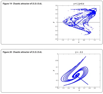
In this case, the chaotic attractor forr=r=  andr=r= . looks like in Figures 

and .

Figure 19 Chaotic attractor of (5.5)-(5.6).

Figure 20 Chaotic attractor of (5.5)-(5.6).

Here we also rewrite system (.)-(.) as follows:

x(t) =  –αx(t–r) +y(t–r), (.)

y(t) =βxt– (r–r)

. (.)

Here we show the chaotic attractor for system (.)-(.). Figure  shows the chaotic attractor whenr=  andr= , while Figure  shows the chaotic attractor of the same

system but withr= . andr= ..

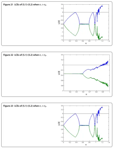
Since the Lyapunov exponent is a good indicator for the existence of chaos [–], we compute the Lyapunov characteristic exponents (LCEs) via the Householder QR-based methods described in []. LCEs play a key role in the study of nonlinear dynamical sys-tems, and they are a measure of sensitivity of solutions of a given dynamical system to small changes in the initial conditions. One feature of chaos is sensitive dependence on initial conditions; for a chaotic dynamical system, at least one LCE must be positive. Since for non-chaotic systems all LCEs are non-positive, the presence of a positive LCE has often been used to help determine if a system is chaotic or not. Figure  shows the LCEs for sys-tem (.)-(.) in the caser>rforβ= . with the initial conditions (x,y) = (, ). With

these parameter values, we find that LCE = . and LCE = –.. While Figure  shows the LCEs for the same system in the caser<rforβ= –. with the same initial

conditions, we find that LCE = . and LCE = –.. Finally, Figure  shows the LCEs for system (.)-(.) in the caser=rfor parameter valuesβ= –. with the same

Figure 21 LCEs of (5.1)-(5.2) whenr1>r2.

Figure 22 LCEs of (5.1)-(5.2) whenr1<r2.

Figure 23 LCEs of (5.1)-(5.2) whenr1=r2.

6 Conclusion

The discontinuous (sectionally continuous) dynamical system of the Henon map describes dynamical properties for different values of the parameters r,r∈R+ when the time

t∈[,T] is continuous. Indeed, the stability of fixed points depends on the values of delay parametersr andr as we have seen. The bifurcation diagrams, as well, depend on the

values of delay parametersrandrand the time interval [,T]. We have also noticed that

the chaotic attractor of the discontinuous (sectionally continuous) Henon system in its different versions is also affected by the change inr,rand the time interval [,T]. On

Competing interests

The authors declare that they have no competing interests.

Authors’ contributions

The authors declare that the study was realized in collaboration with the same responsibility. All authors read and approved the final manuscript.

Author details

1_{Department of Mathematics, Faculty of Science, Alexandria University, Alexandria, Egypt.}2_{Faculty of Education,}

Alexandria University, Alexandria, Egypt.

Acknowledgements

The authors would like to thank the referees of this manuscript for their valuable comments and suggestions.

Received: 9 June 2013 Accepted: 24 March 2014 Published:08 Apr 2014 References

1. El-Sayed, AMA, Nasr, ME: Existence of uniformly stable solutions of nonautonomous discontinuous dynamical systems. J. Egypt. Math. Soc.19(1-2), 91-94 (2011)

2. El-Sayed, AMA, Nasr, ME: On some dynamical properties of discontinuous dynamical systems. Am. Acad. Sch. Res. J.

2(1), 28-32 (2012)

3. El-Sayed, AMA, Nasr, ME: Dynamic properties of the predator-prey discontinuous dynamical system. Z. Naturforsch. A

67a, 57-60 (2012)

4. El-Sayed, AMA, Nasr, ME: On some dynamical properties of the discontinuous dynamical system presents the logistic equation with different delays. i-manag. J. Math.1(1) (2012)

5. El-Sayed, AMA, Nasr, ME: Some dynamic properties of a discontinuous dynamical system. Alex. J. Math.3(1) (2012) 6. El-Sayed, AMA, Nasr, ME: Discontinuous dynamical systems and fractional-orders difference equations. J. Fract. Calc.

Appl.4(12), 1-9 (2013)

7. El-Sayed, AMA, Salman, SM: Chaos and bifurcation of discontinuous dynamical systems with piecewise constant arguments. Malaya J. Mat.1(1), 15-19 (2012)

8. El-Sayed, AMA, Salman, SM: Chaos and bifurcation of discontinuous logistic dynamical system with piecewise constant arguments. Malaya J. Mat.3(1), 14-20 (2013)

9. El-Sayed, AMA, El-Raheem, ZF, Salman, SM: On some dynamics of Duffing dynamical system generated by a semi-discretization process with two different delays. Math. Sci. Lett.3(2), 89-96 (2014)

10. El-Sayed, AMA, Salman, SM: Discontinuous dynamical systems generated by a semi-discretization process. Electron. J. Math. Anal. Appl.1(1), 47-54 (2013)

11. Bilal, S, Ramaswamy, R: The generalized time-delayed Henon map: bifurcations and dynamics. Int. J. Bifurc. Chaos

23(3), 1350045 (2013)

12. Sprott, JC: High-dimensional dynamics in the delayed Henon map. Electron. J. Theor. Phys.3(12), 19-35 (2006) 13. Bohai, NA: Continuous solutions of systems of nonlinear difference equations with continuous arguments and their

properties. Nonlinear Oscil.10(2), 169-175 (2007)

14. da Cruze, JH, Táboas, PZ: Periodic solutions and stability for a singularly perturbed linear delay differential equation. Nonlinear Anal.67, 1657-1667 (2007)

15. Elaydi, SN: An Introduction to Difference Equations, 3rd edn. Undergraduate Texts in Mathematics. Springer, New York (2005)

16. Hale, J: Theory of Functional Differential Equations. Springer, New York (1977) 17. Kuznetsov, YA: Elements of Applied Bifurcation Theory, 3rd edn. Springer, Berlin (2004)

18. Jing, ZJ, Yang, J: Bifurcation and chaos in discrete-time predator-prey system. Chaos Solitons Fractals27, 259-277 (2006)

19. Liu, X, Xiao, D: Complex dynamic behaviors of a discrete-time predator-prey system. Chaos Solitons Fractals32, 80-94 (2007)

20. Wu, G-C, Baleanu, D: Discrete fractional logistic map and its chaos. Nonlinear Dyn.75(1-2), 283-287 (2014) 21. Wu, G-C, Baleanu, D, Zeng, S-D: Discrete chaos in fractional sine and standard maps. Phys. Lett. A (2014).

doi:10.1016/j.physleta.2013.12.010

22. Udwadia, FE, von Bremen, H: A note on the computation of the largestp-Lyapunov characteristic exponents for nonlinear dynamical systems. J. Appl. Math. Comput.114, 205-214 (2000)

10.1186/1687-1847-2014-107