(Received December 7, 2010; Revised November 5, 2011; Accepted November 30, 2011; Online published October 24, 2012)
This study aims to develop a three-dimensional (3D) numerical analysis code for the prediction of driftage behavior during a tsunami. The main features of this code are as follows: (1) it can simulate the six degree-of-freedom motion of driftage in a 3D flow field; (2) it can consider the interaction between fluid flow and driftage motion; and (3) it can compute the impact of the collision with a wall based on the Lagrangian equation of impulsive motion. In this code, we assume that the fluid pressure and viscosity cause driftage motion and that driftage motion affects fluid flow through deformation of the boundary between the fluid and itself. The code was applied to a hydraulic experiment carried out by subjecting a wooden body to an abrupt flow of water. The obtained numerical solution of driftage motion agreed well with the experimental result. It is concluded that our code can be used to successfully predict the behavior of driftage carried by a tsunami.
Key words:Three-dimensional numerical analysis, tsunami, driftage, six degree-of-freedom motion.
1.
Introduction
During the Indian Ocean Tsunami in 2004, rubble, cars, etc., drifted toward coastal areas with the receding waves and destroyed buildings and structures. Rubble from de-stroyed structures was also adrift, causing increased dam-age. To reduce such damage, it is essential to predict the be-havior and collision force of tsunami driftage. Ushijimaet al.(2006) and Kawasakiet al.(2006) proposed methods for the three-dimensional (3D) simulation of tsunami driftage. These methods can simulate driftage behavior accurately by treating the driftage as a fluid; however, they also have to simulate the air flow. In this study, we have developed a numerical method that does not require the simulation of the air flow to predict the driftage behavior across a wide coastal area. Yoneyamaet al.(2002) performed a numeri-cal analysis of the lonumeri-cally high run-up caused by the 1993 Hokkaido-Nansei-Oki seismic tsunami. The wave height calculated by them agreed well with the actual wave height. We believe that the driftage behavior can be simulated with a high degree of accuracy by appending a driftage simula-tion funcsimula-tion to their fluid analysis code. We had devel-oped a vertical two-dimensional (2D) analysis code based on this method, and had verified its validity (Nagashimaet al., 2008). In this study, we developed a new 3D numerical analysis code that can simulate the six degree-of-freedom motion of driftage. We verified the validity of this code by comparing the obtained results with a numerical result and with the results of hydraulics model test.
Copyright cThe Society of Geomagnetism and Earth, Planetary and Space Sci-ences (SGEPSS); The Seismological Society of Japan; The Volcanological Society of Japan; The Geodetic Society of Japan; The Japanese Society for Planetary Sci-ences; TERRAPUB.
doi:10.5047/eps.2011.11.010
2.
Numerical Analysis Method
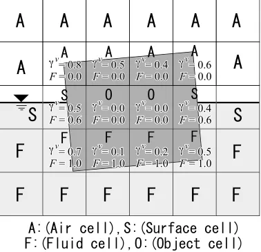
Our method treats the driftage as a rigid body that is set in motion by the gravitational and fluid forces; these forces are determined by a fluid analysis (see Fig. 1). Meanwhile, the fluid analysis treats the driftage as a moving boundary that is expressed in terms of the porosity ratio of the com-putational cellγv and the aperture ratio of the cell surface
γa(see Fig. 2).
The movement of driftage causes a change in the porosity ratio and in the aperture ratio of the computational cell. This change affects the fluid flow; this effect can be expressed by the following continuity equation.
2.1 Basic equations for fluid flow
The basic equations of fluid flow are shown below. •Continuity equation
•Advection equation of fluid ∂γvF
whereuiis the component of flow velocity;gi, the
compo-nent of the external force per unit volume (vector represen-tation isg);p, the pressure;ρ, the density of the fluid;ν, the dynamic viscosity;F, the fluid-filling ratio of the void in a cell;¯, the Reynolds averaging quantity; and , the fluctu-ation in the Reynolds averaging quantity. We also used the
Fig. 1. Drift motion.
Fig. 2. Drift treatment.
followingk-εmodel of turbulent flow to calculate Reynolds stress−uiuj.
−uiuj =
Cμk2 ε
∂ui
∂xj +∂uj
∂xi
−2
3kδi j (4)
∂k ∂t +
1 γv
∂γa
jkuj
∂xj
= ∂
∂xj
ν+Cμk2
σkε
∂k
∂xj
−uiuj∂ui ∂xj −ε
(5)
∂ε ∂t +
1 γv
∂γa
jεuj
∂xj
= ∂
∂xj
ν+Cμk2
σεε
∂ε ∂xj
−Cε1ε
ku
iuj
∂ui
∂xj
−Cε2ε 2
k (6)
wherek(≡uiui/2)is the turbulent energy,ε(≡νui,jui,j)is
the turbulent energy dissipation, andδi j is the Kronecker
delta. The constant numbers in Eqs. (4), (5), and (6) are σk=1.0,σε=1.3,Cε1=1.45,Cε2=1.92,Cμ=0.09.
Our method is based on the SIMPLE method (Patankar and Spalding, 1972); we use discretized equations (Eqs. (1), (2), and (3)) on the Cartesian coordinate system to represent
Fig. 3. Coordinate system for fluid flow and drift rotation.
Fig. 4. Segment and segment surface in a cell.
fluid flow. The definition points of the flow velocity and the others were at the center of the boundary phase between the cells and at the centers of the cells, respectively. The discretizations of time, advective term, and others yielded the forward difference, third-order upwind difference, and centered difference, respectively. Moreover, we discretized Eq. (3) using the volume of fluid (VOF) method (Hirtet al., 1981). We also devised a few countermeasures to conserve fluid volume (Yoneyama, 1998).
2.2 Basic equations of driftage motion
The driftage motion calculation is based on rigid motion analysis. In addition to the Cartesian coordinate system used in fluid analysis, an inertia principal-axis coordinate system is used for the analysis of driftage motion. The coordinate system moves with a driftage, and its origin is the centroid (gravity center) of the driftage (see Fig. 3).
(a) In case of internal cell (b) In case of surface cell
Fig. 5. Pressure calculation.
•Equation of motion of the driftage centroid
mdvg
dt =mg+
k Fprk +
k
Fvisk (7)
•Equation of rotational motion about the driftage centroid
Idωωωωωωωω
dt +ωωωωωωωω×Iωωωωωωωω=
k
rsk× F
pr
k +Fvisk
(8)
wheremis the mass of the driftage,vgis the driftage
cen-troid velocity vector, andFprk andFvisk are the vectors of the
fluid pressure and viscous force, respectively, acting on the segment surface.ωωωωωωωωis an angular velocity vector on the in-ertia principal-axis coordinate system.Iis an inertia tensor that consists of the inertia moment of driftage. rsk is the position vector of the centroid of a segment surface on the inertia principal-axis coordinate system.
2.3 Algorithm of fluid force that acts on driftage 2.3.1 PressureFpr As shown in Eq. (9), the pressure
that acts on a “segment surface” Ppris estimated by using
the cell pressurePc(see Fig. 5).
Ppr= Pc−ρgh=Pc−ρg(rs−rc)z (9)
whereh is the vertical interval between the centroid of a segment surface and the cell center;rs, the position vector
of the centroid of a segment; andrc, the position vector of
the cell center. In this estimation, a hydrostatic pressure is assumed to be acting between the centroid of a segment surface and the cell center. Therefore, the fluid pressure acting on a segment surface is expressed by
Fpr=PprS(−n) . (10)
whereS is the area of a segment surface andn, the normal vector of the surface. In case of a cell including a water surface, a centroid and an area of the submerged part of the segment surface are used for estimation (see Fig. 5(b)).
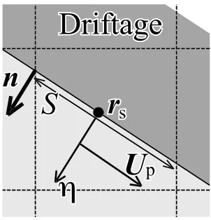
2.3.2 Viscous forceFvis If U(r)is a velocity vector
at a positionr, then the component of the velocity vector parallel to a segment surfaceUpis expressed as follows.
Up =U−(n·U)n (11)
Fig. 6. Viscosity calculation.
If rs is the centroid of a segment surface, then the shear
stress on the surface, ττττττττ(rs) is expressed as follows (see
Fig. 6).
ττττττττ(rs)=μ
∂Up
∂η
r=rs
(12)
whereμ is the viscosity coefficient of the fluid and η, a coordinate axis with originrsthat is directed along a normal
vectorn.
Thus, the viscosity force acting on a segment surfaceFvis
can be expressed as
Fvis =ττττττττ(rs)S =μS
∂Up
∂η
r=rs
. (13)
2.4 Calculation related to collision
When the collision is predicted to occur before the fol-lowing calculation step (betweentand (t+t)), the motion of the driftage is calculated as follows.
i) Calculate the velocity of the driftage centroid,vg, and
Fig. 7. Experimental apparatus used in Case 1.
ii) Calculate the time of the collision occurrence (t + tcol) and the position vector of the collision point on
the inertia principal-axisrcolusingvgandωωωωωωωω.
iii) Calculate the velocity of the driftage centroidvgand
the angular velocity of the inertia principal-axis ωωωωωωωω immediately after collision using the following equa-tions.
wherencolis the normal vector of the collision surface
(wall, bed etc); andJ, the impulse force, given by the following expression.
whereeis the reflection coefficient.
iv) Calculate the position of driftage centroidXgand
rota-tion angle of inertia principal-axisθgat time oft+t
by usingvg,ωωωωωωωω,vgandωωωωωωωω.
In this procedure, FprandFvis is not changed before and after the collision. Equations (14) and (15) are derived from the Lagrangian equation of impulsive motion, which was applied the Newton’s hypothesis.
2.5 Calculation procedure
The calculation procedure is as follows:
i) Read the input data.
ii) Set the boundary condition for flow velocity uni and
pressurepnat timet.
iii) Calculate the turbulence energykn+1, the turbulent
en-ergy dissipationεn+1 , and the eddy viscosityνn+1
t at
timet+t.
iv) Calculate the flow velocityuni+1at timet+t using the discretized form of Eq. (2).
v) Calculate the position and rotation angles of the drif-tage,Xn+1
gi andθ
n+1
g , respectively, at timet+tusing
the discretized forms of Eqs. (8) and (9).
vi) Calculate the void ratio and aperture ratio,γvn+1 and
γan+1
i , respectively, at timet+t.
vii) Calculate the error in the continuity equation Dusing the discretized form of Eq. (1). IfDexceeds the limit Dmax, then correct the pressure pn+1 on the basis of
the solution of the pressure error equation and return to step iv). If not, then proceed to step viii).
viii) Calculate the fluid-filling ratioFn+1at timet+t.
ix) If it is time to stop, then stop the calculation. If not, increase the time and return to step ii).
3.
Application and Discussion
3.1 Case 1: driftage in sea
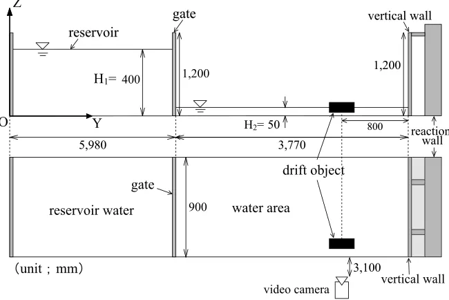
Ikenoet al.(2001) conducted a hydraulic experiment to determine the collision force of an object with a simple ge-ometry drifted by a tsunami; they proposed a formula to de-termine the approximate collision force. Their experimental apparatus is shown in Fig. 7. The model scale is 1/100. The gate was quickly opened, water from the reservoir flowed toward the wall, and the object drifted. The driftage in this case is a wooden object and its specific gravity is 0.5. One side of the experimental flume is made of clear glass and the motion of the driftage was recorded from the glass side using a high-resolution video camera.
The experimental conditions for calculations using our method were as follows: Water levels were H1 = 40 cm,
H2 = 5 cm. The driftage was a cylinder with a diameter
of 8 cm and a height of 20 cm. The initial position of the centroid of this object wasY =8.95 m. The computation conditions are as follows: The grid spacing is 6.5 cm along the direction across the flow, 6 cm along the flow direc-tion, and 3 cm in the vertical direction. The computational time intervalt is 1.0 ×10⁻³ s, The maximum
Fig. 8. Comparison of the trajectory patterns of the driftage obtained in Case 1.
(a)t=0.00 s
(b)t=1.51 s (c)t=2.01 s
(d)t=2.23 s (e)t=3.01 s
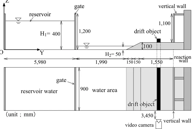
Fig. 10. Experimental apparatus used in Case 2.
fluid densityρ is 1.0×10³ kg/m3, kinematic viscosity ν is 1.0×10⁻⁶m2/s, density of the driftageρ
d is 0.5×10³
kg/m3, and the reflection coefficient between the driftage
and vertical walleis 0.5. For computational purposes, the cylindrical driftage was modeled as an octagonal pillar with cross-sectional area and volume equal to that of the actual cylinder (driftage).
Figure 8 shows the results of a comparison between the vertical 2D trajectory of the driftage obtained by the compu-tation and that obtained in the experiment. In this figure, the trajectories of the centroid of the front-end face (land side) and the rear-end face (sea side) of the driftage are compared. The circles denote the location of the centroid of the front-and rear-end face of the driftage after every 0.5 s from the start of its motion. “×” indicates the location where the driftage collided with the vertical wall.
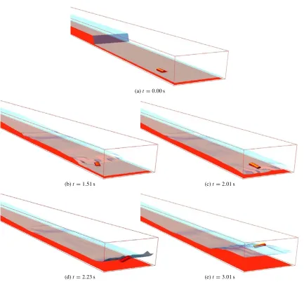
Figure 9 shows examples of the simulation results. The time shown in this figure indicates the time elapsed since the start of the experiment.
As shown in Fig. 8, the computed driftage trajectory, time variation of the position, and point of collision are in good agreement with the corresponding experimental re-sults. Therefore, we concluded that our code can success-fully predict the behavior of driftage in the sea.
3.2 Case 2: driftage on land
Ikeno and Tanaka (2003) conducted another hydraulic experiment to determine the behavior of driftage on land. The experimental apparatus is shown in Fig. 10. This ap-paratus is the same as that in Case 1 with the exception of a 10-cm-high ground segment in the front of the vertical wall. The driftage is a square pillar with side 4.5 cm and height 89 cm. The initial position of the driftage centroid isY =9.02 m. The other experimental and computational conditions are the same as those in Case 1. In the analysis, the bottom surface of the driftage is raised by 0.005 m from the surface of the ground segment. This was done so that the water flowing through the 0.005-m gap would exert an
upward force on the driftage.
Figure 11 shows the results of a comparison between the vertical 2D trajectory of the driftage obtained by the computation and that obtained in the experiment. In this figure, the trajectories of the driftage centroid are compared. The circles and the “×” carry the same meaning as in Fig. 8.
Figure 12 shows examples of the simulation results. As shown in Fig. 11, the computed trajectory elevation of the driftage between the initial position and the vertical wall was higher than the experimental result. Therefore, the collisions that occurred at low elevations in the experiment did not show in the computation results. This difference might be caused by the initial gap between the driftage and the ground surface. In future works, it is necessary to understand the mechanism of initial movement and to find a suitable initial condition.
However, in general, the computed drifting behavior agrees well with the experimental results despite the initial movement problem. Therefore, we concluded that our code can successfully predict the behavior of driftage on land.
4.
Conclusion
The results of our research are summarized as follows: • A numerical analysis code has been developed to
pre-dict the behavior of driftage carried by a tsunami. The main features of the code are as follows.
– It can simulate driftage motion with six degrees-of-freedom in a 3D flow field.
– It can consider the interaction between a fluid flow and a driftage motion.
– It can determine the impact of the collision of driftage with a wall on the basis of the La-grangian equation of impulsive motion.
Fig. 11. Comparison of the trajectory patterns of the driftage obtained in Case 2.
(a)t=0.00 s
(b)t=1.51 s (c)t=2.04 s
(d)t=2.50 s (e)t=3.01 s
paper.
Acknowledgments. The authors are indebted to Dr. Masaaki Ikeno, Central Research Institute of Electric Power Industry, Japan, for kindly supplying his experiment data.
References
Hirt, C. W. and B. D. Nichols, Volume of fluid (VOF) method for the dynamics of free boundaries,J. Comput. Phys.,39, 201–225, 1981.
MICS) for transportation of solid bodies in 3D free-surface flows,J. Hydrau. Coast. Environ. Eng., JSCE,810/II-74, 79–89, 2006. Yoneyama, N., Development of free surface hydraulic analysis code
(FRESH),Nagare (Jpn. Soc. Fluid Mech.),17(3), 1998.
Yoneyama, N., M. Matsuyama, and H. Tanaka, Numerical analysis for locally high runup of 1993 Hokkaido Nansei-oki Seismic Tsunami,J. Hydrau. Coast. Environ. Eng., JSCE,705/II-59, 139–150, 2002.