The dynamical behavior of the earth’s magnetosphere based on laboratory
simulation
R. Rana1, S. Minami1, S. Takechi1, A. I. Podgorny2, and I. M. Podgorny3
1Department of Electrical Engineering, Osaka City University, Osaka 558-0014, Japan 2P. N. Lebdev Physical Institute, Moscow, Russia
3Space Research Institute, Moscow, Russia
(Received May 17, 2004; Revised September 17, 2004; Accepted September 24, 2004)
A laboratory simulation experiment was performed to observe the dynamical behavior of the earth’s magneto-sphere, based upon the earthward electric field measurement in the magnetotail. The simulation was examined to satisfy the MHD scaling laws. The earthward electric field, Ex, is the signature of the current density based on
j ×Bforce in the tail, described by Podgorny (1978). The effect of the solar wind dynamic pressure to the earth-ward electric field,Ex, was investigated. The solar wind density was changed while the other parameters were kept almost constant. It is found that theEx is modulated by the change in the solar wind dynamic pressure. The result also shows that the current continued to flow in the near earth region even after the solar wind had stopped. This result shows a similar resemblance to that of the particle confinement in the radiation belt of the real magnetosphere. Key words: Magnetosphere, solar wind, electric field, magnetic field, current sheet, field aligned current, plasma confinement.
1.
Introduction
For an understanding of the auroral acceleration mecha-nism and substorm formation, it is important to know the magnetospheric current system. Laboratory experiments have been performed by many workers to investigate the magnetosphere phenomena using an intense plasma flow simulating the solar wind and a strong dipole magnetic field simulating the earth (Bosticket al., 1963; Cladiset al., 1964; Kawashima, 1964; Fukushima and Kawashima, 1964; Os-borneet al., 1964; Podgorny, 1976; Birnet al., 1992). The configuration of the field line of the magnetosphere was mea-sured by using a magnetic probe with a uniformly applied ex-ternal magnetic field simulating the IMF by Podgorny (1976) and Baum and Bratenahl (1982). Minami et al.(1977) in-vented a small discharge electrode in order to map the mag-netic field line configuration in the tail region. The more detailed experiments have been done by Minami and Takeya (1985); Minami et al., (1988b) and Minami (1994). Exact scaling of the simulation experiments of the magnetosphere is examined, based on Schindler’s criterion (Shindler, 1969). These experiments have shown the existence of the open and closed magnetosphere. The simulation of the magnetosphere of other planets is also conducted based on the same tech-nologies (Minami et al., 1990). The simulation of differ-ent space phenomena, other than earth’s magnetosphere, has been performed by Minamiet al.(1986, 1988a) and Minami (1994).
The earthward electric field, Ex, was first measured by Minamiet al.(1993) in the laboratory. TheExis generated
Copy right cThe Society of Geomagnetism and Earth, Planetary and Space Sciences (SGEPSS); The Seismological Society of Japan; The Volcanological Society of Japan; The Geodetic Society of Japan; The Japanese Society for Planetary Sciences; TERRA-PUB.
due to Hall Effect because the j ×Bforce is applied to the electrons and the electric field accelerates ions (Podgorny and Podgorny 1992).
TheExis expressed by,
Ex =(Jy/ne)Bz (1)
where:
J=nev (2)
wheren,e,vare carrier charge density, charge and velocity, respectively (Minamiet al., 1993).
The experimental value of the Ex was measured by an electric double probe and the magnetic field was measured by a magnetic probe. The result of experiment showed that the Ex decreases gradually far from the earth because Bz component decreases gradually as shown in Eq. (1). The result by Minamiet al.(1993) also confirmed that the dawn-dusk current is dominantly carried by electrons. If the current is carried by the ions then the polarity ofy-component of tail electric field is completely reversed. The measuredExin the current sheet is relatively accurate and valuable to imagine the distribution of the current,J, in the tail.
The FAC sheets are responsible for the energy transport to the ionosphere. Podgornyet al. (2003) shows that the FAC generator is the earthward electric field, Ex, in the magnetotail. Byusing the satellite measurements it is shown by Podgornyet al.(2003) that there are two sheets flowing away from the ionosphere at low latitude and flowing into the ionosphere at high latitude. The electric field between the two FAC sheets reaches the value of about 150 mV/m. The electric field is directed perpendicular to the FAC sheets. The connection of the FAC in ionosphere is described by Podgornyet al.(2003). They show that the FAC is generated in the magnetotail due to earthward electric field appearance.
(a) (b)
Fig. 1. (a) Outer view of the chamber. (b) Inner view of the chamber.
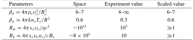
Table 1. The MHD scaling laws.
Parameters Space Experiment value Scaled value βd =4πρoυo2/B
2
o 6–7 4–∞ 6–7
βp =4πknoTo/B2 0.6 0.3 0.6
Rm =4πxoυo/ηc2 ∼1012 103 1 Rh =4πxoυono/c Bo ∼8×10³ 10 1
The electric field in MHD approximation is expressed by
E = −v × B/c + j × B/nec +pe/ne (Podgorny et
al., 2003). The term pressure gradient,pe, is negligible. During a substorm, plasma velocity, v, is directed to sun, and the electric field directed to sun can only be created by the Hall electric field j ×B/nec. The potential drop of this field is projected along the field line from the distance order of 20 RE. Podgornyet al.(2003) described that the normal magnetic fieldBndue to the existence of dipole geomagnetic field exists in entire current sheet in the magnetotail.
2.
Experiment
To simulate the solar wind as a magnetohydrodynamic medium, it is necessary to eliminate electron-neutral colli-sion effects and electron-ion collicolli-sions and to get a high mag-netic Reynolds number, Rm. To get a fine structure of inter-action between the simulated solar wind and the dipole mag-netic field, the ion gyroradius must be small compared with the size of the earth’s magnetosphere. In the experiment, the ion-neutral and ion-ion collisions have been reduced to make a collision-free solar wind. The condition for the ion-mean free paths in the laboratory simulation scaling laws by Bara-nov (1969) is too severe. Therefore the new entity has been added to calculate the ion-mean free path. (1) The simulated solar wind plasma is flowing at a very high speed and the residual neutral particles near the plasma gun expand slowly. During the solar wind and magnetosphere interaction of the duration 30μsec, there is no neutrals particle from the gun in the experimental region. Therefore, electron-neutral colli-sions are neglected. (2) Due to the high plasma velocity, ther-mal velocity is replaced by the drift velocity of the simulated solar wind for the calculation of ion-mean free path. The new equation for effective ion-mean free path, λ∗i, is given
by,
λ∗
i =νi/υi (3)
=νi.Ti/4.78×10−8NiZ2ln (4)
whereνi is the drift velocity. For the plasma density, N, =5×1013cm−3, the electron temperature,T,=10 eV, and
ln,=9, the ion-mean free path,λ∗i, is calculated as,
λ∗
i =20 cm. (5)
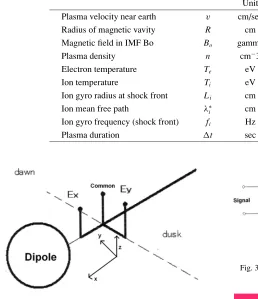
Table 2. The parameters in space and experiment.
Unit Nature Experiments
Plasma velocity near earth v cm/sec 3×10⁷ 3×10⁷
Radius of magnetic vavity R cm 6×10⁷ 4
Magnetic field in IMF Bo Bo gamma 15 107
Plasma density n cm−3 10 1×10¹³
Electron temperature Te eV 10 6
Ion temperature Ti eV 10 5
Ion gyro radius at shock front Li cm 3×10⁷ 6.3×10⁻³
Ion mean free path λ∗i cm 1.3×10⁵ 20
Ion gyro frequency (shock front) fi Hz 100 1.3×10⁸
Plasma duration t sec ≈ ∞ 3×10⁻⁵
Fig. 2. A schematic illustration of the two doubleE-probes located along the sun-earth in the magnetotail.
Table 2 contains the laboratory simulation parameters which have been used in the experiment (Minami et al., 1988).
The experiment was made by using a pulsed artificial hy-drogen plasma flow to simulate the solar wind, produced by a coaxial plasma gun. Figure 1 is the experimental device, used in the simulation experiment. Figure 1(a) is the outer view of the chamber. The size of the vacuum chamber is 160 cm and 70 cm in length and in diameter respectively. Figure 1(b) is the inner view of the vacuum chamber, in which the dipole is inserted from the left side of the chamber. The ap-plied voltage of the plasma gun, VG, is 20 kV and the gun current, IG, is 100 kA. A capacitor bank of capacity 6μF has been used. The size of the simulated earth is 4 cm in diameter. A simulated dipole magnetic field is produced by the coil current, Id,= 600 A. The surface of the dipole is conductively coated for the ionospheric current to flow. The
Idflows for about 1 ms, to create a magnetic field strength of 20 kG at the equator, which is long enough compared with the duration of the solar wind plasma. During the whole ex-periment, the base pressure was kept to 10−5Torr.
The x andz component of electric field, Ex andEy, are measured by two double E-probes located on the sun-earth line in the nightside magnetosphere as shown in Fig. 2. The probes are made of tungsten with a diameter of 1 mm and a length of 2 mm. The probes directed along x andy axis are represented asExandEyrespectively. The separation of the electrodes is 10 mm. In the laboratory experiment, the electron temperature has been measured along the tail and
Fig. 3. The circuit of the photocoupler to measure theExand theEy.
Fig. 4. The photograph of simulated magnetosphere. The simulated solar-wind plasma is coming from the left side and interacting with the dipole magnetic field.
found that the value is almost constant of 5 eV. It can be said that the effect of electron temperature gradient between two points of the double probe is totally negligible for the electric field measurement. Figure 2 is a schematic illustration of the two doubleE-probes.
A high frequency response photocoupler with a light-emitting diode has been used to transfer the signal of Exto eliminate a common mode noise. The overall frequency re-sponse of system is 1μsec. Figure 3 is a diagram of the circuit.
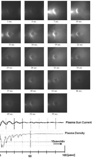
sim-1 sec 4 sec 7 sec 10 sec
13 sec 16 sec 19 sec 22 sec
25 sec 28 sec 31 sec 34 sec
37 sec 40 sec 43 sec 46 sec
49 sec 52 sec 55 sec
Fig. 5. A set of time-resolved photographs of the simulated solar wind interaction with the dipole magnetic field. The two waveform traces show the time variations of the plasma gun current and the solar wind plasma density. This plasma density was measured by a double probe.
ulating the solar wind comes from the left. The luminosity shows that bow-shock is created due to the super sonic flow interaction with the dipole magnetic field. The duration of the main pulsed plasma flow is 30 μsec. During the flow, in every 8 μsec the solar wind dynamic pressure is modu-lated by changing the gun current while the other parameters are kept almost constant. The characteristic time,T, for the plasma to pass through a dayside magnetosphere of 7 cm (corresponding to 10RE in space) is about 1μsec (1 hour in space).
Figure 5 shows a set of time resolved-photographs of the
Fig. 6. The time variations of the earthward electric field,Ex, measured along sun-earth line in the nightside magnetosphere. The time variations of the plasma gun current and the solar wind plasma density are also shown.
3.
Results
3.1 Earthward electric field measurement
A double E-probe is used to measure the Ex. Figure 6 shows time variation of the Exduring the changes in the so-lar wind dynamic pressure. The main plasma gun current, and the solar wind density, measured on sun-earth line off the dipole, are also shown in Fig. 6. The Exhas been mea-sured along the sun-earth line fromx = −2 cm tox = −13 cm in the magnetotail. In the region between x = −7 cm andx = −13 cm, modulation of the Ex is weak compared with the modulation of Ex in the near-earth magnetotail re-gion. The Eq. (1) shows that the Ex is a function of j ×B force. The j ×B force accelerates the plasma along the tail to the earth. The value B in Eq. (1) corresponds to the normal component of magnetic field, Bn, described by Podgorny et al.(2003). The Bn component is responsible for the earthward electric field, Ex, generation. The change in solar wind dynamic pressure strongly modulates the Bn component strength. In the near earth region, the j × B
force strongly modulates due to the change inBncomponent which results in the strong modulation of earthward electric
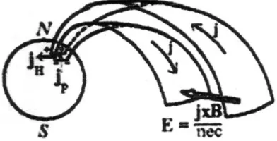
Fig. 7. A schematic illustration of the FAC circuit generated by Hall electric field in the tail current sheet (Podgornyet al., 2003).
Fig. 8. The time variations of the measuredExandEy, atx = −3 cm and−4 cm, show the continuous flow of ring current in the magnetotail before and after the solar wind stopped. The time variations of the plasma gun current and the solar wind plasma density are also shown.
field, Ex, generation. However, in the far-earth region, the strength ofBncomponent is weak therefore the j×Bforce decreases gradually and theExmodulation decreases.
Figure 7 is a schematic illustration of the FAC structure (Podgornyet al., 2003). The current flows along the dawn-dusk direction and closed FAC. TheExcauses charged par-ticles to flow along the field lines. The field line structure described by Podgornyet al.(2003) may have some resem-blance as of the experimental field lines.
3.2 Plasma confinement
Plasma Confinement Time
Distance Along Sun-Earth Line, x, (cm)
Confinement Time (micsec)
Fig. 9. Measured plasma confinement time at different positions along sun-earth line in the magnetotail.
the simulated magnetosphere, and the luminosity is present in the dipole magnetic field even after the solar wind flow disappears.
We calculated the plasma confinement time of the plasma current in the magnetotail using the Bohm diffusion time,tB. The Bohm magnetic field diffusion coefficient, DB, is given by
DB =1/16 kTe/e B (6)
and the plasma confinement time,tB, is expressed as
tB =R2/2DB (7)
where R is the effective radius of the plasma column. The effective radius of the simulated ring current is regarded as about 1 cm. So for a magnetic field of 1 kG at the equator with the electron temperature, Te,= 10 eV and an effective radius, R,= 1 cm, the value of Bohm magnetic field diffusion coefficient,DB, is as follows;
DB =6×104cm2s−1 (8)
and the plasma confinement time is calculated as:
tB =10μsec. (9)
Figure 9 is the measured plasma confinement time in the magnetotail at different positions, along sun-earth line. The confinement time is determined by the time when theEx de-creases to 10% of the maximum value at each position. It can be seen that the plasma confinement time decreases gradu-ally as the position goes down to the tail. The confinement time at x = −3 cm andx = −4 cm is consistent with the time expressed by the Bohm diffusion time.
4.
Conclusion
This experiment suggests that the dynamical behavior of the Ex in the tail is related to the structural change of the magnetosphere. Due to a change in the dynamical pressure of the solar wind, it is observed that the size of the magne-tosphere shrinks and expands several times repeatedly. This modulation depth of about 50% is controlled by the change of the sheet current density in the tail. The current density is modulated by the shrinking of the magnetosphere.
The continuous flow of the tail current near the earth after the solarwind disappearance is related to the effective current confinement of the ring current particles. The confinement time is consistent with the predicted Bohm diffusion time of the plasma in the magnetic field. These results suggest some effective plasma confinement, as of the dipole configuration of the real magnetosphere. This result also supports the usefulness of the dipole confinement experiment for fusion research (Kesneret al., 1998)
References
Baranov, P. J., Simulation of flow of interplanetary plasma past the magne-tosphere of the earth or planets,Cosmic Res.,7, 98–104, 1969. Baum, P. J. and A. Bartenahl, The laboratory magnetosphere,Geophys. Res.
Lett.,9, 435–438, 1982.
Birn, J., G. Yur, H. U. Rahman, and S. Minami, On the termination of the closed field line region of the magnetotail,J. Geophys. Res.,97, 14883– 14840, 1992.
Bostick, W. H., M. Brettschneider, and H. Byfield, Plasma flow around three-dimensional dipole,J. Geophys. Res.,68, 263–269, 1963. Cladis, J. B., T. D. Miller, and J. R. Baskett, Interaction of supersonic plasma
stream with a dipole magnetic field,J. Geophys. Res.,69, 463–469, 1964. Fukushima, N. and N. Kawashima, Model experiments and neutral phenom-ena of interaction of solar plasma stream with geomagnetic field, Rep. Ionos, Space Res. Japan, 18, 4, 1964.
Kawashima, N., The interaction of plasma stream with three-dimensional magnetic dipole,J. Phys. Soc.,18, 59–64, 1964.
Kesner, J., L. Bromberg, D. Garnier, and M. Mauel, Plasma confinement in a magnetic dipole, ICP/09, 17th Fusion Energy Conference, Oct 19–24, 1998.
Minami, S., Effects of the local interstellar medium magnetic filed on the structure of the heliosphere: A laboratory simulation,Geophys. Res. Lett., 21, 81–84, 1994.
Minami, S. and Y. Takeya, Flow of artificial plasma in a simulated magne-tosphere: Evidence of direct interplanetary magnetic field control of the magnetosphere,J. Geophys. Res.,90, 9503–9518, 1985.
Minami, S., Y. Hirose, and Y. Takeya, Simulation experiment of twined plasma produced by powered double probe in the tail region of the mag-netosphere, Mem. of Fac. of Eng. Osaka City Uni., 18, 27–36, 1977. Minami, S., P. J. Baum, G. Kamin, and R. S. White, Laboratory formation
of a simulated comet,Geophys. Res. Lett.,13, 884–887, 1986. Minami, S., P. J. Baum, G. Kamin, and R. S. White, Laboratory comet
simulation experiments, inLaboratory and Space Plasmas,edited by H. Kikuchi, 621 pp., Springer Verlag, New York, 1988a.
Minami, S., P. J. Baum, G. Kamin, and Y. Takeya, Laboratory behavior of a plasma plume injected into the magnetized plasma flow,J. Geomag. Geoelectr.,40, 1283–1302, 1988b.
Minami, S., K. Hashimoto, and Y. Takeya, Dipole tilt angle effect on the magnetosphere of Neptune—a laboratory simulation,Geophys. Res. Lett.,17, 896–899, 1990.
Minami, S., I. M. Podgorny, and A. I. Podgorny, Laboratory evidence of Earthward electric field in the magnetotail current Sheet,Geophys. Res. Lett.,20(1), 9–12, 1993.
Osborne, F. J. F., M. P. Bachynski, and J. V. Gore, Laboratory studies of the variation of the magnetosphere,J. Geophys. Res.,69, 4441, 1964. Podgorny, I. M., Laboratory experiments (Plasma intrusion into the
mag-netic field), Space Research Institute, Rep. Pr.-225, 1976.
Podgorny, I. M., Current sheet formation, in Fundamental of Cosmic Physics,4, pp. 1, 1978.
Podgorny, A. I. and I. M. Podgorny, A solar flare model including the formation and destruction of the current sheet in the corona,Solar Phys., 139, 125–145, 1992.
Podgorny, I. M., A. I. Podgorny, S. Minami, and R. Rana, The mechanism of energy release and field-aligned current during the substorms and solar flares,Advances in Polar Upper Atmosphere Research,17, 77–83, 2003. Schindler, K., Laboratory experiments related to the solarwind and the
mag-netosphere,Rev. of Geophys.,7(1,2), 51–75, 1969.