R E S E A R C H
Open Access
A refined affine approximation method of
multiplication for range analysis in
word-length optimization
Ruiyi Sun, Yan Zhang
*and Aijiao Cui
Abstract
Affine arithmetic (AA) is widely used in range analysis in word-length optimization of hardware designs. To reduce the uncertainty in the AA and achieve efficient and accurate range analysis of multiplication, this paper presents a novel refined affine approximation method, Approximation Affine based on Space Extreme Estimation (AASEE). The affine form of multiplication is divided into two parts. The first part is the approximate affine form of the operation. In the second part, the equivalent affine form of the estimated range of the difference, which is introduced by the approximation, is represented by an extra noise symbol. In AASEE, it is proven that the proposed approximate affine form is the closest to the result of multiplication based on linear geometry. The proposed equivalent affine form of AASEE is more accurate since the extreme value theory of multivariable functions is used to minimize the difference between the result of multiplication and the approximate affine form. The computational complexity of AASEE is the same as that of trivial range estimation (AATRE) and lower than that of Chebyshev approximation (AACHA). The proposed affine form of multiplication is demonstrated with polynomial approximation, B-splines, and multivariate polynomial functions. In experiments, the average of the ranges derived by AASEE is 59% and 89% of that by AATRE and AACHA, respectively. The integer bits derived by AASEE are 2 and 1 b less than that by AATRE and AACHA at most, respectively.
Keywords: Word-length optimization; Range analysis; Affine approximation; Accuracy; Uncertainty analysis
1 Introduction
As a method of representing real numbers, floating point can support a wide dynamic range and high precision of values. It has been thus commonly used in signal pro-cessing, such as image propro-cessing, speech propro-cessing, and digital signals processing, to represent signals. When these applications are implemented on hardware for high speed and stability, the signals need to be represented in fixed point to optimize the performance of area, power, and speed of the hardware. Hence, the values in floating-point need to be converted to those in fixed floating-point. This process is named as word-length optimization. Its goal is to achieve optimal system performance while satisfying the specification on the system output precision. Word-length optimization involves range analysis and precision
*Correspondence: [email protected]
Key Laboratory of Network Oriented Intelligent Computation, Harbin Institute of Technology Shenzhen Graduate School, Xili, Shenzhen 518055, China
analysis. The former one is to find the minimum word length of the integer part of the value, while the latter one focuses on the optimization of the fractional part of the word length.
Word-length optimization has been proven to be an NP-hard problem [1]. It can be usually classified into dynamic analysis [2-7] and static analysis [8-20]. By analyzing a large set of stimuli signals, dynamic analysis is applicable to all types of systems. However, it will take long time on simulation to provide sufficient confidence. Also, the pre-cision for the signals without simulation cannot be guar-anteed. Comparatively, the static analysis is an automated and efficient word-length optimization method and more applicable to large designs when compared to dynamic analysis. The static analysis mainly uses the characteristics of the input signals to estimate the word length conser-vatively, which can result in overestimation [12] to some extent. As a part of word-length optimization, the range analysis can also been classified in the same way.
Affine arithmetic (AA) [21] is often used for range analysis in static analysis. In AA, every signal must be represented in an affine form, which is a first-degree polynomial. As AA tracks the correlations among range intervals of signals, it can provide more accurate word-length range. This makes it suitable for range analysis of the result of linear operations. It is noted that besides linear operations, nonlinear operations, such as multipli-cation, are also involved in hardware operations, typically in linear time invariant (LTI) systems. AA cannot pro-vide an exact affine form for nonlinear operations. To solve this problem, Stolfi and de Figueiredo [22] proposed affine approximation methods for multiplication, which include trivial range estimation (AATRE) and Chebyshev approximation (AACHA). AATRE is efficient for compu-tation, but the range produced by it can be four times of real range at most. The accumulation of the uncertainty of all signals in the computational chain may result in an error explosion, which is unacceptable in application. Such overestimation obviously cannot satisfy the accuracy requirement of the system, which limits the application of AATRE in large systems. The uncertainty of AACHA is less than AATRE, however, it is too complex to be used in large systems. Since LTI operations are accurately cov-ered by AA, the proposed method is applied in the field of the range analysis of word-length optimization in this paper.
A novel affine approximation method, Approximation Affine based on Space Extreme Estimation (AASEE), is proposed to reduce the uncertainty of multiplication and achieve an accurate and efficient range analysis of multi-plication in this paper. To analyze the uncertainty conve-niently, we use two parts to divide the different parts of all the approximation methods for multiplication, which include AATRE, AACHA, and AASEE. The first part is named as approximate affine form, which is approximated to the nonlinear operation. The second part is named as equivalent affine form, which is the equivalent affine form of the estimated range of the difference between the result of multiplication and the approximate affine form. The more accurate the two parts are, the more accurate the approximation method is. Based on linear geometry [23], it is proven that the proposed approximate affine form is the closest to the result of multiplication. To derive the equivalent affine form, we use the extreme value theory of multivariable functions [24] to estimate the upper and lower bounds of the difference in space, and the differ-ence is introduced by the approximation of the first part. The uncertainty of the proposed method is minimized. The accuracy of the resulting affine form by AASEE is higher than that by AATRE and averagely higher than that by AACHA. Meanwhile, the computational complexity of AASEE is equivalent to that of AATRE and lower than that of AACHA.
The rest of this paper is organized as follows. Back-ground of range analysis for multiplication is presented in Section 2. Section 3 presents the method of derivation of the two parts for multiplication. The refined affine form of multiplication, AASEE, is presented in next section. In Section 5, we compare the computational complexity and the accuracy among AASEE to AATRE and AACHA. The case studies and experimental results are demonstrated in Section 6. Section 7 concludes the paper.
2 Background 2.1 Related work
Interval arithmetic (IA) and affine arithmetic (AA) have been widely used in range analysis in word-length opti-mization.
IA [25] is a range arithmetic theory which is firstly presented by Moore in 1962. Cmar [2] employs it for range analysis of digital signal processing (DSP) systems. Carreras [20] presents a method based on IA. To reduce the oversized word length, the method provides the prob-ability density functions that can be used when some truncation must be performed due to constraints in the specification. IA is not suitable for most real-world appli-cations, since it could lead to drastic overestimation of the true range.
AA [21] is proposed to overcome the weakness of IA by Stolfi in 1993. In [8,9], Fang uses AA to analyze word-length optimization. Both range and precision are represented by the same affine form, which limits the optimization. Pu and Ha [10] also use AA for word-length optimization. Simultaneously, they use two differ-ent affine forms for range analysis and precision analysis, respectively, and achieve more refined result of word-length optimization. Similarly, Lee et al. [11] develop an automatic optimization approach, which is called MiniBit, to produce accuracy-guaranteed solutions, and area is minimized while meeting an error constraint. Osborne [12] uses both IA and AA for range analysis for different situations. Computation using either of the two methods in the design is time-consuming. The problem of over-estimation is serious due to the approximation of the nonlinear operations.
Since AA cannot be used in the systems with infinite number of loops, an improved approach, quantized AA (QAA), has been proposed in [13] for linear time-invariant systems with feedback loops. This method can provide fast and tight estimation of the evolution of large sets of numerical inputs, using only an affine-based simulation, but it does not provide the exact bounds.
parameterNin theN-level simplified affine approxima-tion (N-SAA). This method is faster than AACHA and more accurate than AATRE, but it is more complex than AATRE. Furthermore, it is troublesome to choose a suit-ableN. A method of range analysis is proposed by Pang [26]. This method combines methods of IA, AATRE, and arithmetic transform (AT); and the result of the method is more accurate than AATRE, while the CPU implemen-tation time is longer than AATRE. To deal with appli-cations from the scientific computing domain, Kinsman [17,18] uses the computational methods based on Satisfi-ability Modulo Theory. Search efficiency of this method is improved leading to tighter bounds and thus smaller word length.
For all the existing methods, the accuracy of approxi-mation is improved at the expense of the computational complexity. This paper presents an affine approximation method for multiplication, which achieves better trade-off between accuracy and computational complexity.
2.2 Range analysis
Range analysis involves studying the data range of every signal and minimizing the integer word lengths for signals on the premise that the signals in the design have enough bits to accommodate this range. The range of signalxis represented byx=[xmin,xmax], where the two real num-bers,xminandxmax, denote the lower and upper bounds ofx, respectively. The required integer part of the word length for signalx, which is represented as IWLx, can be derived by:
IWLx=
log2(|x|max) +α, |x|max≥1
1, |x|max<1
.
where|x|max=max(|xmin|,|xmax|) and
α=
1, mod(log2(xmax), 1)=0 2, mod(log2(xmax), 1)=0 .
(1)
In (1), all the signals in the design are assumed to be expressed as signed numbers, and the sign bit is taken into account in IWLx. According to (1), once the range of a signal is decided, the integer part of word length of the signal can be derived.
2.3 Affine arithmetic
AA is widely applied for range analysis. In AA, an uncer-tain signalx is represented by an affine form as a first-degree polynomial [22]:
ˆ
x=x0+x1ε1+x2ε2+· · ·+xnεn, whereεi=[−1, 1] . (2)
For the signal x, x0 is the central value, andεi is the
ith noise symbol.εi denotes an independent uncertainty
source that contributes to the total uncertainty of the signalx, andxiis its coefficient.
The upper and lower bounds for the range ofxcan be represented as
xmax=x0 +
n
i=1
|xi|, xmin=x0−
n
i=1
|xi|. (3)
Withxminandxmax, the input intervalx¯=[xmin,xmax] can be converted into an equivalent affine form as (4), using only one independent noise symbol.
ˆ
x=x0+x1ε1,
withx0=
xmax+xmin
2 , x1=
xmax−xmin
2 .
(4)
AA can keep correlations among the signals of the com-putational chain by contributing the sample noise symbol εito each signal [22].
For multiplication, AATRE and AACHA are typical approximation methods.
The affine form of AATRE is
ˆ
xyˆ=x0y0+
n
i=1
(x0yi+y0xi)εi+ n
i=1
|xi|
n
i=1
|yi|εn+1.
(5)
SupposeM1 =max(n1,n2), in whichn1andn2denote the number of the noise symbol, whose coefficient is nonzero, ofxˆandyˆ, respectively. The computational com-plexity of AATRE isO(M1).
AACHA provides a better approximation result, but it is more complex. The affine form of AACHA is
ˆ
xyˆ=x0y0+
n
i=1
(x0yi+y0xi)εi+
a+b
2 +
b−a
2 εn+1, (6)
whereaandbdenote the minimum and the maximum of the range of
n
i=1 xiεi
n i=1
yiεi
. SupposeM2=n1+n2.
The complexity of computing the both extremal values,a andb, isO(M2logM2). AsM1 ≤ M2, the computational complexity of AATRE is lower than that of AACHA [22].
2.4 Extreme value theory
The proposed approximation is based on the extreme value theory of multivariable functions [24].
the local maxima and the local minima. Hessian matrix of is indefinite whenHfα is neither positive semidefinite nor negative semidefinite. IfHfα is positive definite, then fα is a local minimum point. IfHfα is negative definite, then fα is a local maximum point. IfH
fα is indefinite, thenfα is neither a local maximum nor a local minimum. It is a saddle point. Otherwise,fαis not utilized in this paper.
The principal minor determinants are used to deter-mine if a matrix is positive or negative definite or semidefinite.
It is necessary and sufficient for a positive semidefinite matrix that all the principal minor determinants of the matrix are nonnegative real numbers.
It is necessary and sufficient for a negative semidefinite matrix that all the odd order principal minor determi-nants of the matrix are non-positive real numbers and all the even order principal minor determinants of the matrix are nonnegative real numbers.
3 Derivation of the two parts for multiplication A generic nonlinear operationz ← f(xˆ,ˆy) proposed in [22] can be described by (8):
z=f(x0+x1ε1+ · · · +xnεn,y0+y1ε1+ · · · +ynεn) =f∗(ε1,. . .,εn).
(8)
Since the operationf is nonlinear,f∗(ε1,. . .,εn)cannot be expressed exactly as an affine combination of the noise symbols,εi. Under this case, an approximate affine form of the operation, which is represented asfz, must be used to approximatef∗(ε1,. . .,εn). The difference introduced by this approximation,df = f∗−fz, can be expressed by an equivalent affine form of the estimated range of the dif-ference, which is represented asdˆ. Hence, the affine form ofzcan be expressed as
ˆ
The computational complexity of computing the true range ofdfis very high in a practical application. The esti-mated range ofdf is utilized instead of the true range. Sup-posedmaxanddmindenote the upper and lower bounds of the estimated range ofdf, respectively. According to (4), thedˆcan be expressed as (11)
With (10) and (11), the affine form ofz can be repre-sented as
For multiplication,zcan be expressed as
z=x0y0+x0
The first three items of (13) form an affine form and the last term is a quadratic term. Its affine form can also be represented as (12).
In the existing affine approximation methods of AATRE and AACHA, dmax and dmin are estimated in the XY plane. In these methods, the same noise symbol of dif-ferent variables is considered to be independent. Hence, the range ofdˆ is much larger than that ofdf. The differ-ence betweendˆ anddf will propagate tozˆ and result in uncertainty.
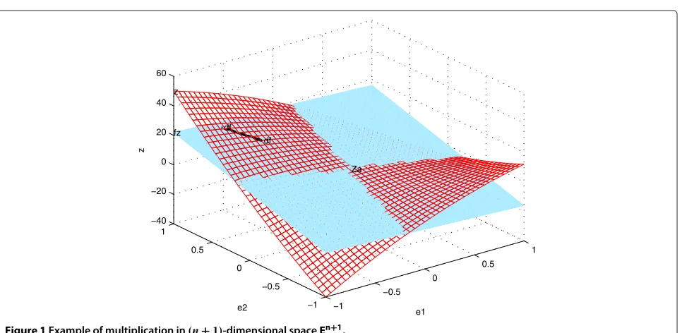
(n+1)-dimensional hyperplane and a nonlinear polyno-mial function denotes a(n+1)-dimensional space curved surface. The approximate affine form in (10) denotes a (n+1)-dimensional hyperplane inEn+1. Each hyperplane inEn+1can be viewed as a parallel translation of a tangent hyperplane at a certain point of(n+1)-dimensional space curved surface. Hence, all possible approximate affine forms for zcan be regarded as the(n+1)-dimensional tangent hyperplanes at all points of(n+1)-dimensional space curved surface inEn+1. The translation amount is taken into account indf, which is approximated bydˆ. In spaceEn+1,df can be viewed as the function of the dis-tance between the points of space curved surface and the tangent hyperplane.
Figure 1 shows an example of xˆ = 1+ε1+5ε2 and
ˆ
y=3−6ε1+ε2. The space is labeled as(ε1,ε2,z). The red mesh surface represents the functionz= ˆxyˆ =(1+ε1+ 5ε2)(3−6ε1+ε2). The blue plane represents the tangent planefz,z = 3−3ε1+16ε2, at the pointzα = (0, 0, 3). All the possible approximate affine forms forzare the tan-gent planes of all the points.df is a function of distance betweenzandfz.
Here we usefzα in (18) to represent the tangent hyper-plane at the pointzα =(ε1α,εα2,. . .,εnα). Then, the possible approximate affine form can be represented asfzα, too.
fzα =zα+zε 1(ε1−ε
α
1)+zε2(ε2−ε
α
2)+· · ·+zεn(εn−ε
α
n). (18)
In (18),zεnare the partial derivatives ofzwith respect to the variablesεnat the pointzα.
With the estimated range ofdf, the maximum absolute error ofdf can be expressed as
ea=max(|dmax|,|dmin|). (19)
To reduce the uncertainty,fzmust be the most closed to the result of multiplication. Hence,fzis the tangent hyper-plane whose maximum absolute error is minimum among that of all the possible affine formfzα, that is,
ea(fz)=min(ea(fzα)). (20)
The geometrical meaning of fz denotes the tangent hyperplane whose maximum absolute error is minimized. fz is derived by the range ofdf, while dˆ is the equiva-lent affine form ofdf. It is very complex to compute the true range of df. Withdˆ in (11), the uncertainty in AA for nonlinear operations is generated due to the difference between the true range ofdf and the estimated range of
df.
It is much tighter and easier to estimate range ofdf in En+1 space than in theXY plane. Based on the extreme value theory of multivariable functions, the estimated range ofdf in AASEE is derived.
With more accuratedmaxanddmin,fzanddˆcan be cal-culated more precisely, and AASEE can achieve a refined affine approximation result.
In the next sections, the estimated range ofdf will be derived firstly, and the two parts will be derived later.
−1
−0.5 0
0.5 1
−1 −0.5 0 0.5 1 −40 −20 0 20 40 60
e1 Za
df
e2 df z
fz
z
4 AASEE for multiplication 4.1 Estimated range of the difference
For multiplication, which is expressed as (13), the value of zat the pointzαis
The partial derivatives ofzwith respect to the variableεi at the pointzαare
Upon substitution for zα andzεi, the tangent hyper-planefzαcan be expressed as
The difference between the tangent hyperplanefzα and (n+1)-dimensional quadratic surfacezis
df =z−fzα =
Suppose demax and demin denote the estimated maxi-mum and minimaxi-mum of the function value at the domain boundary respectively, and dfimax anddfimin denote the local maxima and the local minima, respectively. The esti-mated maximum and minimum of multivariable function df,dmaxanddmin, can be expressed as
dmax=max(demax,dfimax), (25)
dmin=min(demin,dfimin). (26)
According to (24), the function value at the domain boundary,dfe, is represented by
dfe= Under this case, for the first item, it is always positive
when i = j. Hence, the estimated function value at the domain boundary,de, is expressed as
de=
Hence, the maximum and minimum of de, demax and deminare derived as
demax=
To simply compare,dfimaxanddfiminin (25) and (26) can be expressed as
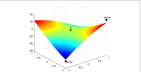
As the example in Section 3, Figure 2 shows the function ofdf = −6(ε1−0.1)2−29(ε1−0.1)(ε2−0.1)+5(ε2−0.1)2 whenεα1 = 0.1 andε2α = 0.1. The estimated maximum and minimum ofdf at the domain boundary,demax and demin, are also marked in the figure. Since the value of εi in (27) are substituted by ∀εi = ±1,demax is larger than the maximum of df and demin is smaller than the minimum.
−1
−0.5 0
0.5 1
−1 −0.5 0 0.5 1 −60 −40 −20 0 20 40
demax
P
demin
Figure 2df,demax, anddeminof the example in Section 3.
Hessian matrix of functiondf = n i,j=1
xiyj(εi−εαi)(εj−εjα) is
H = ⎡ ⎢ ⎢ ⎢ ⎢ ⎢ ⎢ ⎢ ⎢ ⎣
∂2df
∂ε2 1
∂2df
∂ε1ε2 · · ·
∂2df
∂ε1εn
∂2df
∂ε2ε1
∂2df
∂ε22 · · · ∂2df
∂ε2εn · · · · · · · ·
∂2d f
∂εnε1
∂2d f
∂εnε2 · · ·
∂2d f
∂ε2 n
⎤ ⎥ ⎥ ⎥ ⎥ ⎥ ⎥ ⎥ ⎥ ⎦
= ⎡ ⎢ ⎢ ⎢ ⎢ ⎢ ⎢ ⎣
2x1y1 x1y2+x2y1 x1y3+x3y1 · · · x1y2+x2y1 2x2y2 x2y3+x3y2 · · · x1y3+x3y1 x2y3+x3y2 2x3y3 · · ·
· · · ·
· · · ·
x1yn+xny1 x2yn+xny2 x3yn+xny3 · · · ⎤ ⎥ ⎥ ⎥ ⎥ ⎥ ⎥ ⎦ .
(33)
From (33), we can see thatHis independent ofεi. It is a expression ofxiandyi. This means thatHis same for all the points in the domain.
To determine if H is positive or negative definite or semidefinite, its principal minor determinants are derived as
D0=2xiyi (34)
D1=
2xiyi xiyj+xjyi
xiyj+xjyi 2xjyj
= −(xiyj−xjyi)2 (35)
D2=D3= · · · =Dn=0,
where 1≤i<j≤n. (36)
As introduced in Section 2.4,His a positive semidefinite matrix, iff it satisfies
∀xiyi≥0,∀xiyj=xjyi, for 1≤i<j≤n. (37)
His a negative semidefinite matrix, iff it satisfies
∀xiyi≥0,∃xiyj=xjyi, for 1≤i<j≤n. (38)
If it satisfies neither (37) nor (38), which means it satis-fies (39),His an indefinite matrix as
∃xiyi<0, for 1≤i≤n. (39)
According to (37), (38), and (39), we can comparedemax, demin,dfimax, anddfimin, which are expressed as (29), (30), (31), and (32), respectively. Based on (25) and (26),dmax anddmincan be identified.
Lemma 1.The estimated maximum of function df, dmax
equals to the estimated maximum of the function value at the domain boundary, and the estimated minimum of function df, dmin equals to the estimated minimum of
the function value at the domain boundary. This can be expressed as
dmax=demax dmin=demin. (40)
For∃xiyi < 0, (39) is satisfied andH is indefinite. The stationary point is a saddle point, such as the pointPin Figure 2. Neitherdfimaxnordfiminexists indf, that is,
dmax=demax dmin=demin. (41)
According to (41), Lemma 1 can be proven in this case. For∀xiyi ≥ 0,H may be positive semidefinite or neg-ative semidefinite. df may have local minima or local maxima under this condition.
As εi =[−1, 1], the following inequalities are estab-If a local maximum lies at zα, the difference between demaxanddfimaxis
According to (25) and (46), we can prove that
dmax=demax. (47)
Similarly, if a local minimum lies at zα, the difference betweendeminanddfiminis
demin−dfimin≤ −
According to (26) and (49), we can prove that
dmin=demin. (50)
As (47) and (50) are established, Lemma 1 can be proven in the case of∀x1y1≥0.
Combining these two cases, Lemma 1 is proven.
According to Lemma 1,dmaxanddminat a pointzαcan be computed asdemaxanddeminin (29) and (30).
4.2 Expression of the approximate affine form in AASEE Lemma 2.When fzrepresents a tangent hyperplane at
the point z0=z
0=(0, 0,. . ., 0), it satisfies (20).
Proof. According to Lemma 1, (29), and (30), the maxi-mum absolute error ofdf is
ea= |
So the maximum absolute error between the tangent hyperplanefz0 at the point z0 = z0 = (0, 0,. . ., 0)and (n+1)-dimensional quadratic surfacezis
ea(z0)= | maximum absolute error between the tangent hyperplane fzα at pointzα and(n+1)-dimensional quadratic surface whose maximum absolute error is minimized.
It is proven that the chosenfzis a tangent hyperplane at the pointz0=z0=(0, 0,. . ., 0).
4.3 Expression of the equivalent affine form in AASEE According to (55), thedf between the tangent hyperplane
fz0and the quadratic surface is
df = n
i,j=1
xiyjεiεj. (56)
According to Lemma 1, (29), and (30), the estimated maximum and estimated minimum ofdf,dmaxanddmin can be expressed as
dmax= demax=
By combining the two cases,demaxanddeminare rewrit-ten as
According to (11), the affine form ofdˆcan be expressed as
The affine form ofdˆcan be expressed as
ˆ
d= 1 2x1y1+
1
2|x1y1|ε2. (65)
4.4 Formulary of AASEE
According to (12), the affine form of AASEE for multipli-cation is
It is impossible to obtain the exact affine form for mul-tiplication in AA. The result of mulmul-tiplication must be approximated to an affine form. Using εi as the input arguments, the uncertainty of multiplication in AASEE is reduced. The proposedfzis the most closed to the result of multiplication among all the possible approximate affine forms, and the upper and lower bounds ofdˆin AASEE are much closer to true bounds ofdf. Hence, the uncertainty in AASEE is smaller than that in AATRE and AACHA. Formed by suchfzanddˆ, AASEE creates a refined affine form of multiplication.
5 Comparison of AASEE to AATRE and AACHA 5.1 Computational complexity
The computational complexity of an expression is deter-mined by its most complex item. For n > 1, the most complex item is the coefficient of εn+1. To make the analysis convenient, we transform this coefficient:
n
The computational complexity of the minuend isO(M1), whereM1 is defined in Section 2.3, while the computa-tional complexity of the subtrahend is less thanO(M1).
Hence, the computational complexity of AASEE is O(M1). We can see that it is the same as that of AATRE and is lower than that of AACHA.
5.2 Accuracy
For AATRE,dˆ = n
i=1| xi|n
i=1|
yi|εn+1. In this method, the
same noise symbol of different variables is considered to be independent. The range of thisdˆis
−
n
i=1
|xi|
n
i=1
|yi|, n
i=1
|xi|
n
i=1
|yi|
. (69)
It is much larger than the range ofdˆby AASEE, which is expressed in (62) and (64).
In AACHA,dˆ = a+2b + b−2aεn+1, where aandb are represented the estimated range of dˆ. In this method, a polygon inXY plane is used to findaandb. The domain of xˆyˆ is bounded by the polygon. However, the polygon is larger than the true domain, and all the same noise symbols of different variables are not taken into account together.
All the same noise symbols of different variables are considered together bydˆ of AASEE. It is more accurate thandˆ of AATRE. In the most cases, it is more accurate thandˆof AACHA, too.
6 Case studies
The following nonlinear system cases are used to demon-strate the efficiency of the proposed refined affine form of multiplication. These cases are commonly used in sig-nal processing. The first two cases are univariate cases and come from [11]. The rest of cases are multivariate polynomial functions and come from [27-29].
6.1 Introduction of the cases
Case 1. Polynomial approximation. The first case study is that degree-four polynomial for the approximation of y=ln(1+x), wherex=[0, 1]. Horner’s rule evaluates the polynomial
y=(((−0.0550x+0.2168)x−0.4645)x+0.9956)x+0.0001,
where the coefficients are obtained by polynomial curve fitting technique.
Case 2. B-splines Uniform cubic B-splines are com-monly used for image warping [30]. Basic functionsB0,B1, B2, andB3in B-spline are defined as
B0(u)= 1 6(1−u)
3, B 1(u)=
1 6(3u
3−6u2+4),
B2(u)= 1 6(−3u
3+3u2+3u+1), B
3(u)= − u3 6 ,
whereu=[0, 1].
Case 3. Multivariate polynomial functions.In the third case, eight multivariate polynomial functions are exam-ined. They are as follows:
1. Savitzky-Golay filter:
f1(X)=7x31−984x32−76x21x2+92x1x22+7x21
−39x1x2−46x22+7x1−46x2−75
where the input range:X=[−2, 2]2
2. Image rejection unit:
f2(X)=16384
x41+x42+64767x21−x22+x1−x2
+57344x1x2(x1−x2)
where the input range:X=[0, 1]2
3. A random function:
f3(X)=(x1−1)(x1+2)(x2+1)(x2−2)x23
where the input range:X=[−2, 2]3
4. Mitchell function:
f4(X)=4
x41+x22+x232+17x21x22+x23
−20x21+x22+x23+17
where the input range:X=[−2, 2]3
5. Matyas function:
f5(X)=0.26(x21+x22)−0.48x1x2
where the input range:X=[−100, 100]2
6. Three-hump function:
f6(X)=12x21−6.3x41+x61+6x2(x2−x1)
where the input range:X=[−10, 10]2
7. Goldstein-Price function:
f7(X)=
1+(x1+x2+1)2
19−14x1+3x21−14x2
+6x1x2+3x22
×30+(2x1−3x2)2
×18−32x1+12x21+48x2−36x1x2+27x22
where the input range:X=[−2, 2]2
8. Ratscheck function:
f8(X)=4x21−2.1x41+ 1 3x
6
1+x1x2−4x22+4x42
where the input range:X=[−100, 100]2
6.2 Analysis of case 1
For the input range x =[0, 1], equivalent affine form is ˆ
x = 0.5+0.5ε1. For case 1, the intermediate and output signals are defined as
y1= −0.0550x+0.2168, y2=y1x−0.4645, y3=y2x+0.9956, y=y3x+0.0001.
Using AATRE, the affine forms of intermediate and output are
y1=0.1893−0.0275ε1,
y2= −0.36985+0.0809ε1+0.01375ε2,
y3=0.81068−0.14448ε1+0.00688ε2+0.04733ε3, y=0.4054+0.3331ε1+0.0034ε2+0.0237ε3+0.0993ε4.
Using AACHA, the affine forms of intermediate and output are
y1=0.1893−0.0275ε1,
y2= −0.3768+0.0809ε1+0.0069ε2,
y3=0.8291−0.1479ε1+0.0034ε2+0.0220ε3,
y=0.3761+0.3406ε1+0.0017ε2+0.0110ε3+0.0436ε4.
Using AASEE, the affine forms of intermediate and output are
y1=0.1893−0.0275ε1,
y2= −0.37673+0.0809ε1+0.00688ε2,
y3=0.84769−0.14791ε1+0.00344ε2+0.00344ε3, y=0.34999+0.34989ε1+0.00172(ε2+ε3)+0.00344ε4.
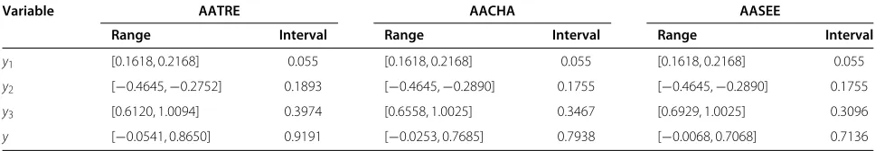
Table 1 shows the variable ranges and the range inter-vals, (ymax −ymin), of intermediates and output by the three methods. The true range ofylies in [0, 0.6931], and the range interval of output is 0.6931. SupposeR(T),R(C), andR(A) are represented as the ratios of range interval obtained by AATRE, AACHA, and AASEE to the true range interval, respectively. The closer this ratio converges to 1, the more accurate the method is. In this case, as R(T) = 1.33,R(C) = 1.15, and R(A) = 1.03, we can see the range by AASEE is closer to the true range than AATRE and AACHA.
6.3 Comparison of range and computational complexity by the three cases
The output ranges by the three methods of case 2 and case 3 can be obtained according to the process of case 1.
Table 2 demonstrates the ranges and the integer word lengths by AASEE and comparison among AATRE, AACHA and AASEE. Columnc.funshows the case study and the function of the row. The true output ranges, which are used as reference values, are obtained by numerical
method or nonlinear programming technique, which are time-consuming and are not practical to solve the true bounds for large number of signals. From the table, we can see that the ranges, which are derived by AASEE, cover the true ranges and they are smaller than those by AATRE, for all the functions. For these thirteen functions, the ranges, which are derived by AASEE, are smaller than those by AACHA for nine functions, and equal to those by AACHA for two functions. According to (1), the inte-ger word length can be decided by the range. The inteinte-ger word-length, which is derived by AASEE, is 2 b less than that by AATRE and 1 b less than that by AACHA, at most. Comparing with AATRE, AASEE and AACHA can save 0.54 b on average.
To calculate the estimated range of df, the values of ∃εi = ±1,∀i = 1, 2,. . .,n in (27) are substituted by ∀εi = ±1 in AASEE. The difference between the esti-mated range and the true range ofdf is introduced by this approximation. In most of the applications, the estimated ranges, which are computed by AASEE, are closer than those by AACHA. However, the estimated minimum and maximum ofxˆyˆon the boundary of the polygon are inde-pendent of the value ofεi. In some applications such as functionsf2andf8in Table 2, the results by AASEE are almost the same as those by AACHA.
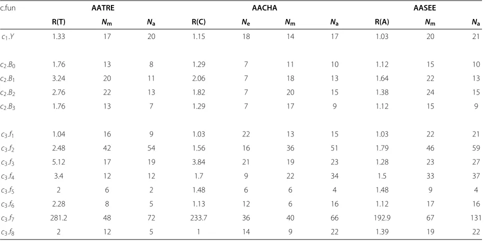
In Table 3, ratios of range intervals and the computa-tional complexity are compared among AATRE, AACHA, and AASEE. The computational complexity is calculated from the numbers of multiplications and additions. For AACHA, the extreme value of a quadratic function in one variable on a bounded interval needs to be calculated. Nm, Na, andNe denote the numbers of multiplications, additions and the extreme value computations of each case, respectively. Table 3 shows thatR(T)values are from 1.04 to 281.2,R(C)are from 1.03 to 233.7, andR(A)are from 1.03 to 192.9. The ratios ofR(A)toR(T)andR(C) show the accuracy of AASEE compared to AATRE and AACHA, respectively. The average ratios can be used to evaluate the accuracy of the affine approximation meth-ods. The ratios of R(A) to R(T) are from 0.18 to 0.99, and the average of these ratios is 0.59. The ratios ofR(A) to R(C) are from 0.33 to 1.17, and the average of these ratios is 0.89. For these 13 cases, on average, the accu-racy of AASEE is 1.69 times than that of AATRE and 1.12
Table 1 Comparison of ranges and range intervals for every variable of the three methods for case 1
Variable AATRE AACHA AASEE
Range Interval Range Interval Range Interval
y1 [0.1618, 0.2168] 0.055 [0.1618, 0.2168] 0.055 [0.1618, 0.2168] 0.055
y2 [−0.4645,−0.2752] 0.1893 [−0.4645,−0.2890] 0.1755 [−0.4645,−0.2890] 0.1755
y3 [0.6120, 1.0094] 0.3974 [0.6558, 1.0025] 0.3467 [0.6929, 1.0025] 0.3096
Table 2 Comparison of analytical ranges and bits by the three methods
c.fun True output AATRE AACHA AASEE
Range Bits Range Bits Range Bits Range Bits
c1.Y [0, 0.6931] 1 [−0.0541, 0.8650] 1 [−0.0253, 0.7685] 1 [−0.0068, 0.7068] 1
c2.B0 [ 0, 0.17] 1 [−0.13, 0.17] 1 [−0.05, 0.17] 1 [−0.02, 0.17] 1
c2.B1 [ 0.17, 0.67] 1 [−0.33, 1.29] 2 [−0.05, 0.98] 1 [ 0.10, 0.92] 1
c2.B2 [ 0.17, 0.67] 1 [−0.21, 1.17] 2 [−0.02, 0.89] 1 [ 0.04, 0.73] 1
c2.B3 [−0.17, 0] 1 [−0.17, 0.13] 1 [−0.17, 0.05] 1 [−0.17, 0.02] 1
c3.f1 [−9453, 9303] 15 [−9821, 9671] 15 [−9793, 9487] 15 [−9793, 9487] 15
c3.f2 [−5.51e4, 8.79e4] 18 [−1.75e5, 1.79e5] 19 [−0.95e5, 1.28e5] 18 [−1.15e5, 1.41e5] 19
c3.f3 [−36, 64] 8 [−256, 256] 10 [−192, 192] 9 [−64, 64] 8
c3.f4 [−8, 641] 11 [−1087, 1121] 12 [−223, 881] 11 [−335, 641] 11
c3.f5 [ 0, 104] 15 [−104, 104] 15 [−4800, 104] 15 [−4800, 104] 15
c3.f6 [ 0, 0.94e6] 21 [−1.07e6, 1.07e6] 22 [−0.06e6, 1.00e6] 21 [−0.11e6, 0.94e6] 21
c3.f7 [ 3, 1.01e6] 21 [−1.42e8, 1.42e8] 29 [−1.23e8, 1.13e8] 28 [−9.87e7, 9.61e7] 28
c3.f8 [−1.03, 3.3e11] 40 [−3.3e11, 3.3e11] 40 [−2.1e8, 3.3e11] 40 [−4.2e10, 3.3e11] 40
c.fun, case study and the function of the row.
times than that of AACHA. The extreme value computa-tion, which is only necessary for AACHA, of the quadratic function is the most complex and time-consuming among the operations. Hence, the computational complexity of AACHA is much higher than that of AATRE and AASEE. The increase rate of the number of multiplications,Nm, by AASEE to AATRE is from 0.091 to 1.75, and the average
is 0.450. The increase rate of the number of multiplica-tions,Nm, by AASEE to AACHA is from 0.2 to 1.833, and the average is 0.567. The increase rate of the number of additions, Na, by AASEE to AATRE is from 0.05 to 3.4, and the average is 0.944. The increase rate of the num-ber of additions,Na, by AASEE to AACHA is from 0 to 0.985, and the average is 0.157. The numbers of
multipli-Table 3 Comparison of range ratios and computational complexity by the three methods
c.fun AATRE AACHA AASEE
R(T) Nm Na R(C) Ne Nm Na R(A) Nm Na
c1.Y 1.33 17 20 1.15 18 14 17 1.03 20 21
c2.B0 1.76 13 8 1.29 7 11 10 1.12 15 10
c2.B1 3.24 20 11 2.06 7 18 13 1.64 22 13
c2.B2 2.76 22 13 1.82 7 20 15 1.38 24 15
c2.B3 1.76 13 7 1.29 7 17 9 1.12 15 9
c3.f1 1.04 16 9 1.03 22 13 15 1.03 22 21
c3.f2 2.48 42 54 1.56 16 36 51 1.79 46 59
c3.f3 5.12 17 19 3.84 21 19 23 1.28 23 27
c3.f4 3.4 12 12 1.7 9 22 34 1.5 33 37
c3.f5 2 6 2 1.48 6 6 4 1.48 9 4
c3.f6 2.28 8 5 1.13 12 6 16 1.12 17 16
c3.f7 281.2 48 72 233.7 36 40 66 192.9 67 131
c3.f8 2 12 5 1 14 9 22 1.39 19 22
4 8 12 16 20 24 28 32 2000
4000 6000 8000 10000 12000 14000
Target Precision[bits]
Area[slices]
AATRE
AACHA
AASEE
Figure 3Area variation forc3.f3with increasing target precision.
cations and additions of AASEE are increased a few. As shown in Table 3, AACHA is slightly more accurate for functionsc3.f2andc3.f8, but the computational complexity of AACHA is much higher than that of AASEE.
6.4 Comparison of the design cost by the three methods To compare the design cost, the system area by the three methods, the fractional word lengths are obtained by the precise analysis in [11]. Typically, we select the case of a random function of case 3,c3.f3, for this section. The design of c3.f3 is synthesized on Xilinx Xc2vp30-7ff896 FPGA device (Xilinx, San Jose, CA, USA).
Figure 3 shows the area variation forc3.f3with increas-ing target precision. It can be seen that the area, which is calculated by AASEE, is less than that by AATRE and AACHA, and the area difference between them is increas-ing with the target precision. This difference is from 265 to
729 with the target precision increased. Such optimization of integer word length can save area.
Figure 4 shows the percentage area saving of AASEE over AATRE at different target precision for c3.f3. The percentage area saving is from 14.34% to 5.62% with the target precision increased. Generally, we obtain increased relative saving for lower precision.
7 Conclusions
This paper presents a novel affine approximation method for multiplication, Approximation Affine based on Space Extreme Estimation. In this method, an extra noise sym-bol is added to an approximated affine form.
To reduce the uncertainty in AA, we derive this method in the (n+ 1)-dimensional space En+1. In space En+1, approximate affine form can be regarded as the tangent hyperplane at a certain point of(n+1)-dimensional space
4 8 12 16 20 24 28 32
0 2 4 6 8 10 12 14 16
Target Precision[bits]
Area Saving[%]
curved surface. Using the linear geometry, it is proven that thefzof AASEE is the closest to the result of multiplication among all the possible approximate affine forms. Taking εi as the input arguments, all the same noise symbols of different variables are taken into account together. Hence, the uncertainty ofdˆ of AASEE is reduced. Based on the extreme value theory of multivariable functions, we can prove that the range of thisdˆcovers the true range of the difference introduced by approximation and much tighter than that by AATRE and AACHA.
The uncertainty in AASEE is much smaller than that in AATRE and AACHA on average. At the same time, the computational complexity of AASEE is the same as that of AATRE and lower than that of AACHA.
In the case studies, the accuracy of AASEE is 1.69 times than that of AATRE and 1.12 times than that of AACHA on average. The integer word length, which is derived by AASEE, is 2 b less than that by AATRE and 1 b less than that by AACHA, at most. For the case ofc3.f3, the area, which is computed by AASEE, is less than that by AATRE and AACHA, and the percentage area saving of AASEE over AATRE is from 14.34% to 5.62% with the target precision increased.
Competing interests
The authors declare that they have no competing interests.
Received: 8 June 2013 Accepted: 10 March 2014 Published: 22 March 2014
References
1. G Constantinides, G Woeginger, The complexity of multiple wordlength assignment. Appl. Math. Lett.15(2), 137–140 (2002)
2. R Cmar, L Rijnders, P Schaumont, S Vernalde, I Bolsens, A methodology and design environment for DSP ASIC fixed point refinement, in
Proceedings of Design, Automation and Test in Europe(IEEE Computer
Society, Munich, 09–12 March 1999), pp. 271–276
3. K Kum, W Sung, Combined word-length optimization and high level synthesis of digital signal processing systems. IEEE Trans.
Computer-Aided Design Integr. Circuits Syst.20(8), 921–930 (2001) 4. S Roy, P Banerjee, An algorithm for trading off quantization error with
hardware resources for MATLAB-based FPGA design. IEEE Trans. Comput.
54(7), 886–896 (2005)
5. A Mallik, D Sinha, H Zhou, Low-power optimization by smart bit-width allocation in a SystmC-based ASIC design environment. IEEE Trans. Computer-Aided Design Integr. Circuits Syst.26(3), 447–455 (2007) 6. G Caffarena, C Carreras, JA Lopez, SQNR estimation of fixed-point DSP
algorithms. Eurasip J. Adv. Signal Process.21, 1–12 (2010)
7. A Banciu, E Casseau, D Menard, Stochastic modeling for floating-point to fixed-point conversion, inProceedings of IEEE Workshop on Signal
Processing Systems (SiPS)(IEEE Computer Society, Beirut, 4–7 October
2011), pp. 180–185
8. CF Fang, R Rutenbar, M Puschel, T Chen, Toward efficient static analysis of finite-precision effects in DSP applications via affine arithmetic modeling, inProceedings of Design Automation Conference, Institute of Electrical and
Electronics Engineers Inc.(Anaheim, 2–6 June 2003), pp. 496–501
9. CF Fang, R Rutenbar, Fast, accurate static analysis for fixed-point finite-precision effects in DSP designs, inProceedings of International Conference on Computer-Aided Design, Institute of Electrical and Electronics
Engineers Inc.(San Jose, 9–13 November 2003), pp. 275–282
10. Y Pu, Y Ha, An automated, efficient and static bit-width optimization methodology towards maximum bit-width-to-error tradeoff with affine arithmetic model, inProceedings of Asia and South Pacific Design Automation Conference, Institute of Electrical and Electronics Engineers Inc. (Yokohama, 24–27 January 2006), pp. 886–891
11. DU Lee, AA Gaffar, RC Cheung, O Mencer, W Luk, GA Constantinides, Accuracy guaranteed bit-width optimisation. IEEE Trans. Computer-Aided Design Integr. Circuits Syst.25(10), 1990–2000 (2006)
12. WG Osborne, JGF Coutinho, W Luk, O Mencer, Instrumented multi-stage word-length optimization, inProceedings of IEEE International Conference on Field-Programmable Technology, Institute of Electrical and Electronics
Engineers Inc.(Kitakyushu, 12–14 December 2007), pp. 89–96
13. JA Lopez, C Carreras, O Nieto-Taladriz, Improved interval-based characterization of fixed-point LTI systems with feedback loops. IEEE Trans. Computer-Aided Design Integr. Circuits Syst.2(11), 1923–1933 (2007) 14. L Zhang, Y Zhang, W Zhou, Tradeoff between approximation accuracy
and complexity for range analysis using affine arithmetic. J. Signal Process. Syst.61(3), 279–291 (2010)
15. O Sarbishei, K Radecka, Z Zilic, Analytical optimization of bit-widths in fixed-point LTI systems. IEEE Trans. Computer-Aided Design Integr. Circuits Syst.31(3), 343–355 (2012)
16. R Rocher, D Menard, P Scalart, Analytical approach for numerical accuracy estimation of fixed-point systems based on smooth operations. IEEE Trans. Circuits Syst. I, Reg. Papers.59(10), 2326–2339 (2012)
17. AB Kinsman, N Nicolici, Bit-width allocation for hardware accelerators for scientific computing using SAT-modulo theory. IEEE Trans.
Computer-Aided Design Integr. Circuits Syst.29(3), 406–413 (2010) 18. AB Kinsman, N Nicolici, Computational vector-magnitude-based range
determination for scientific abstract data types. IEEE Trans. Comput.
60(11), 1652–1663 (2011)
19. SA Wadekar, AC Parker, Accuracy sensitive word-length selection for algorithm optimization, inProceedings of the International Conference on Computer Design: VLSI in Computers and Processors, 1998. ICCD ‘98, Institute of Electrical and Electronics Engineers Inc.(Austin, 5–7 October 1998), pp. 54–61
20. C Carreras, JA Lopez, O Nieto-Taladriz, Bit-width selection for data-path implementations, inProceedings of the 12th International Symposium on
System Synthesis, 1999(IEEE Computer Society, Boca Raton, 1–4
November 1999), pp. 114–119
21. JLD Comba, J Stolfi, Affine arithmetic and its applications to computer graphics, inProceedings of SIBGRAPI’93 - VI Simposio Brasileiro de
Computacao Grafica e Processamento de Imagens(IEEE Computer Society,
Recife, 20–22 October 1993), pp. 9–18
22. J Stolfi, LH de Figueiredo (eds), Affine arithmetic, inSelf-Validated
Numerical Methods and Applications(Monograph for 21st Brazilian
Mathematics Colloquium, IMPA, Rio de Janeiro, Brazil, 1997), pp. 70–74 23. K Huang, H Yee, Improved tangent hyperplane method for transient
stability studies [of power systems], inProceedings of APSCOM-91
Conference, Institution of Electrical Engineers(Hong Kong, 5–8 November
1991), pp. 363–366
24. E Eivind, TS Gustavsen,GRA6035 Mathematics(BI Norwegian Business School, Oslo, 2010)
25. R Moore,Interval Analysis(Prentice-Hall, New Jersey, 1966)
26. Y Pang, K Radecka, An efficient algorithm of performing range analysis for fixed-point arithmetic circuits based on SAT checking, inProceedings of
IEEE International Symposium on Circuits and Systems (ISCAS)(IEEE
Computer Society, Rio de Janeiro, 15–18 May 2011), pp. 1736–1739 27. N Shekhar, P Kalla, F Enescu, Equivalence verification of arithmetic
datapaths with multiple word-length operands, inProceedings of Design,
Automation and Test in Europe(IEEE Computer Society, Munich, 6–10
March 2006), pp. 824–829
28. S Gopalakrishnan, P Kalla, MB Meredith, F Enescu, Finding linear building-blocks for RTL synthesis of polynomial datapaths with fixed-size bit-vectors, inProceedings of International Conference on Computer-Aided Design, Institute of Electrical and Electronics Engineers Inc.(San Jose, 5–8 November 2007), pp. 143–148
Conference on Computer Graphics and Virtual Reality(CSREA Press, Las Vegas, 26–29 June 2006), pp. 196–204
30. J Jiang, W Luk, D Rueckert, FPGA-based computation of free-form deformations in medical image registration, inProceedings of IEEE International Conference on Field-Programmable Technology 2003 (IEEE Computer Society, Tokyo, 15–17 December 2003), pp. 234–241
doi:10.1186/1687-6180-2014-36
Cite this article as:Sunet al.:A refined affine approximation method of multiplication for range analysis in word-length optimization.EURASIP Journal on Advances in Signal Processing20142014:36.
Submit your manuscript to a
journal and benefi t from:
7 Convenient online submission
7 Rigorous peer review
7 Immediate publication on acceptance
7 Open access: articles freely available online
7 High visibility within the fi eld
7 Retaining the copyright to your article