Approximate analysis of discrete-time tandem queueing networks with customer loss

Approximate Analysis of

Discrete-Time Tandem Queueing

Networks with Customer Loss

Dooyeong Park

Hany G. Perros

Center for Communications and Signal Processing

Department of Computer Science

North Carolina State University

Approximate Analysis of Discrete-time Tandem

Queueing Networks with Customer Loss

*

Dooyeong Park

Department of Eletrical and Computer Engineering, and

Center for Communications and Signal Processing

North Carolina State University

Raleigh, NC 27695

Harry G. Perro!

Department of Computer Science, and

Center for Communications and Signal Processing

North Carolina State University

Raleigh, NC 27695

Ab,tract- We first approximate the departure process of an IBP /Geo/l/K queue

by an Interrupted Bernoulli Process (IBP). We consider several different approxima-tion models and their accuracy is examined through extensive validaapproxima-tion tests. These models are then used in a simple decomposition algorithm to analyze a tandem config-uration of finite capacity queues with customer loss. The decomposition algorithm is validated by comparing it against simulation and it i. shown to have a good accuracy.

1

Introduction

In recent years there has been a lot of interest in the development of high-speed

communi-cation networks. The most promising design for high-speed networks is the Asynchronous

Transfer Mode (ATM). The need for performance evaluation of ATM networks has given rise

to a widespread in terest for the analysis of discrete- time queueing systems. Discrete- time

single server queues with or without finite capacity have been extensively analyzed. For a

review of relevant results see Pujolle and Petros [10]. However, little has been done for the

analysis of networks of discrete-time finite capacity queues.

A network of discrete-time finite capacity queues can be used to model the queueing

within an ATM switch, or the queueing within a network of ATM switches. Two different

assumptions can be made regarding such a network:(l) A customer gets lost when it arrives

to a full queue.(2) A customer cannot start its service until there is space in the destination

queue. This is similar to the blocking-before-service mechanism that has been extensively

studied in continuous-time queueing networks of finite capacity queues. In

telecommunica-tion systems, this mechanism is often referred to as back pressure.

The external arrival process to the network is assumed to be bursty. Typically, a bursty

arrival process is represented by an Interrupted Bernoulli Process (IBP). In an IBP, we have

a geometrically distributed period during which no arrivals occur, followed by a

geomet-rically distributed period during which arrivals occur in a Bernoulli fashion. The IBP is

a special case of the Markov Modulated Bernoulli Process (MMBP), which has a slightly

more complex structure and it captures the notion of the burstiness and the correlation of

successive interarrival times.

In this paper, we analyze a tandem queueing network of discrete-time finite capacity

queues with customer 108s. The arrival process to the first queues is assumed to be an IBP.

The service times at each queue are assumed to be geometrically distributed. The choice

of the geometric distribution was motivated by ATM networks. In general, a service time

as celQ is constant, and therefore the transmission time is const an t as well. However, in

some ATM switch architectures a cell may be re-transmitted several times due to possible

collisions with other cells. In this case, the total transmission time is typically modelled

by a geometric _distribution. Queueing networks of discrete-time finite capacity queues with

customer loss do not lend themselves to an exact analysis. However, they can be ana.lyzed

approximately using the notion of decomposition. That is, the network is decomposed into

individual queues, and each queue is then analyzed separately. The most important aspect of

such a decomposition is the characterization of the arrival process to an intermediate queue.

In continuous-time queueing networks, typically, such as an arrival process is characterized

approximately by a two-phased Coxian distribution, or by a more general phased-type

dis-tribution. Also, it has been characterized by a general distribution defined by the mean and

squared coefficient of variation. In this paper, the departure process from one queue, which

becomes the arrival process to the next downstream queue is characterized approximately

by an IBP. Various fitting models, motivated by the method of moments, are examined and

compared. These models are then used in the approximate analysis of a tandem queueing

network with discrete-time finite capacity queues.

The interdeparture distribution of a discrete-time GI/G/l queue has been obtained by

Tran-Gia [11] using the Fast Fourier Transform. He also derived the idle period

distribu-tion from the equilibrium distribudistribu-tion of the virtual unfinished work. Ohba, Murata and

Miyahara [8] analyzed a discrete-time single-server queue with the following three arrival

streams: 1) arrivals with a general interdeparture time distribution, 2) Bernoulli arrivals in

batches, and 3) IBP. Discrete-time queueing networks have been analyzed by Morrison [6],

Hsu and Burke [3], Ohba, Murata, and Miyahara [8] and Pujolle [9] assuming infinite

capac-ity queues. Bhargava et

a1

[1] and Bocharov and Albores [2] analyzed tandem configurations

of finite capacity queues with customer 108S, hut in continuous-time. Finally, Morris and

Perros [5] analyzed an ATM switch architecture, which basically involved the analysis of a

discrete-time tandem configuration of finite capacity queues with blocking-before-service.

I-p

:

l-q

Figure 1: The Markov chain for an IBP

The generating function of the interdeparture time of an IBP /Geo/l/K queue is obtained

in section 3. In section 4, we present various fitting models for characterizing the departure

process as an IBP and examine their accuracy. In section 5, we analyze a tandem

configura-tion of finite capacity queues with cell loss using some of the approximaconfigura-tion models obtained

in section 4. The approximate results are compared against simulation in section 5, and

conclusions are given in section 6. We note that in accordance with the terminology of ATM

networks, we shall refer to a customer as a cell.

2

The Interrupted Bernoulli Process

The Interrupted Bernoulli Process (IBP) is defined over a slotted (discrete-time) time axis

and it comprises two states, an active state and an idle state, which alternate. The time

the process spends in each state is geometrically distributed. Arrivals occur in a Bernoulli

fashion when the process is in the active state. No arrival occurs if the process is in the idle

state. Given that the nrocess is in the active state (or idle state) at slot i, it will remain in

the same state in the next slot i

+

1 with probability p(or q),or will change to the idle state (or active state) with probability 1 - p (or 1 - q). The transitions between the active and

idle states are governed by a two state Markov chain as shown in Figure 1. During the active

state, a slot contains a cell with probability Q. a=l means that every busy slot contains a

cell.

Let t be the interarrival time of a cell. It can be shown that the mean interarrival time,

arrivals, ClBP are as follows (see

[7]):

E{t} 2-p-q

a(1 - q) ,

Var(t) E{t}2

=

1

+

a [(

1-

p)(p

+

q) -

1]

(2 -

p - q)2 .

(1)

(2)

The average arrival rate, i.e. the probability that any slot contains a cell, PrBP is given by

a(l - q)

PrBP

=

2 .

-p-q (3)

By varying p and q, we can increase the traffic and at the same time change the burstiness

of the process.

3

The Departure Process of an IBP /Geo/l/K Queue

Let us consider a discrete-time single server queue. Let K be the maximum capacity of the

queue. The service time is defined over a slotted time axis. For presentation purposes, a slot

will be referred to as a service slot. A service always starts at the beginning of a service slot

and the service time is assumed to be a geometric number of service slots with parameter tr,

The arrival process is also defined over a slotted time axis with the same slot size, and it is

assumed to be an IBP with parameters PA, qA, and QA. The boundaries of the slots of the

arrival process is assumed to be in-between the boundaries of the service slots (as shown in

Figure 2). An arriving cell to an empty queue cannot start its service until the beginning

of the next service slot, even though the server is free at the time instant of its arrival. A

departure is assumed to take place just before the end of service slot. Finally, as it will be

seen below we examine this queue at the boundary of each service slot.

In order to analyze the departure process of an IBP /Geo/l/K, we first need to obtain its

slot n

Arrival

slot

n+1

Departure

Figure 2: The arrival and the departure time instants

states for the queue length at the end of every service slot, and subsequently we generate

the rate matrix Q. The stationary probability vector x is then obtained by solving the

linear equations xQ

=

o.

We define the state of the queue by the variables

(s,n).

Variable

s represents the state of the arrival process at the end of a service slot and it takes the

values: 0 if the arrival process is in the idle state, 1 if the arrival process is in the active

state. Variable n indicates the number of cells in the system at the end of a service slot. We

have n=O,l, ..,K, where K is the capacity of the system including the cell in service. Using

the stationary probability vectorx, that can be obtained numerically as described above, we

compute the generating function of the probability distribution of the interdeparture time

of the IBP /Geo/l/K queue as follows.

Let I be a random variable representing the time the server is idle (i.e. the system is idle). This is the time elapsing from the moment a departure occurs to the end of service

slot during which an arrival occurs. Also, let S be a random variable representing the service

time, and let D be a random variable representing the interdeparture time. These random

variables are discrete-time and they take values which are integer multiples of a service slot.

Let us consider two consecutive departure instants corresponding to the two departures of

the (m - l)st and mth customer. The interdeparture interval D is equal to the sum of a

case

1

mel .~ Departure

o

P+(s,n>O)

~fIII::t--- S

o 0 ~

1

0 ~

tim. .lot

m-~hDeparture

case 2

Arrival

P(s,n>O)

I - t - O + C I - - S

tc:I"---D----~ tim• •lo~

mel .1: Departure m-1:h Departure

Figure 3: The interdeparture time

empty system, or it is equal to a service time if the system is not empty after the (m - 1)st

departure. These two cases are shown in Figure 3. I can be expressed as follows:

1 -

p+

(0, 0) -

P+(

1,0)

P+(O,O) P+(l,O)

(4)

where 1₀, II is a random variable indicating the time elapsing from the moment a departure

occurs leaving the system in state (0,0) respectively(1,0) to the end of the service slot during

where an arrival occurs. P+(~,n) is the probability that immediately after a departure the

system is in the state [s,n).

10' II'

and P+[s,n) can be obtained as follows:

(1 - qA)aA qA

(1 - qA)(l -

(lA)

(5)

1

1

+

1

0

1

+

1

1

PAaA 1- PA

PA(1 -

(lA)

P+(s,n)

=

Pr{The system is in state (s,n)

I

a departure has occurred}

=

Pr{The system is in (s,n) and a departure has occurred}_{Pr{A depart ure occurs}}

P+(O,O)

=

(1 - u)[qAP(O, 1)

+

(1 - PA)P(I, 1)] (1 - u)[1 - P(O,O) - P(I,O)]

qAP(O, 1)

+

(1 - PA)P(I, 1)

(7)

=

_{1 - P(O,O) - P(1,O)}

P+(l,O)

=

(1 - qA)(I -

OA)P(O,

1)

+

PA(1 - oA)P(l,

1)

(8)

1 - P(O,O) - P(l, 0)

By taking the z-transform of the equation (5) and (6) we can get:

where 10(z) and 11(z) are the z-transforms of 10 and II' respectively. Using (4), (7), (8),

(9) and (10) we can obtain the following expression for

I(z),

the. generating function of I:

I(z)

=

1 - P+(O,O) - P+(l,O)

+

P+(O,O)Io(z)

+

P+(1,0)I

1(z)

We define D( z) as the generating function of the probability distribution of the

interde-parture time. We haveD=S+I. Since S and I are independent,

D(z)

=

E{zD}

=

8(z)1(z),

where S(z) is the generating functions of S, and it is equal to S(z)

=

(~=:~J:. Thus, we have

where

D(z)

=

a3z3

+

a2 z 2

+

al z

a2

=

_{(1 -}

U){(PA

+

qA)[(I- OA)P+(O,O)

+

P+(I,O) -

_1]

+

OA[P+(O,O)

+

PAl}

at

=

(1 - _{0-)[1 -} P+(O,0) - P+(I, 0)]

b3

=

-0-(1 - QA)(PA

+

qA - 1)

b2

=

(1 -

OA)(PA

+

qA -

₁₎

+

U[qA

+

PA(1 - OA)]

bt

=

-[0-

+

qA

+

PA(1 - QA)].

The moments of the time between successive departures can be obtained by differentiating

D(z) given by (11). In particular, the mean interdeparture time E{D} and the squared

coefficient of variation of the interdeparture time C2 , are as follows:

where

E{D}

= D'(l),

02 = Var(D)

E{D}2

D"(l)

+

D'(l) - [D'(I)]2

-[D'(I)]2

(12)

(13)

D'(l)

D"(l)

=

1

+

P+(O,O)

[(1 -

QA)(1 -

PA - qA)

+

1]

+

P+(l,O)) [2 - PA - qA]

1 - QA

QA(l -

qA) QA(l - qA)

__ +( )

[2(1 -

QA)(PA

+

qA -

l)[QA(1 -

qA)

+

PA(1 - aA)

+

qA -

4]]

P

0,

°

[oA(l -

qA)]2

+

[2(1 -

PA - qA) 2(2 - PA - qA)[(1 - QA)(PA

+

2qA - 2) - qA]]

+P

(1 .ft) oA(1 _

qA)

-

[OA(1 - qA)]2

2

[P+(O,O)(1 -

QA)(l -

PA - qA)

+

1 P+(1,0)(2 - PA - qA)]

+

1 - tT oA(1 -

qA)

+

<lA(1 - qA)

[

2[qA

+

PA(l - QA)]]

20'

+P+(O,O)

[<lA(l _

qA)]2

+

(1 _

u)2'

The link utilization, p, i.e., the probability that any slot contains a cell is:

1

and the third moment of the interdeparture time,

E{D

3} , is:

E{D3_}

=

_{D"'(1)+3D"(1)+D'(1)}

D'''(1)

+

~[3(C2

+

1) - 2p]

p2 (15)

The probability distribution of the interdeparture time can be obtained by inverting

the generating function,

D{z).

This is done as follows (see Kobayashi [4]). Let Pi be the

probability that the interdeparture time is equal to i slots. Then, we have

D(z)

3

Laiz i

i=O

3

L

bizi

i=O

where bo= l . Multiplying both sides by the denominator and then equating the coefficients

of zi on both sides, we obtain the following set of linear difference equations:

min{3,i} { . · _ 0 1 2 3

~ b a, I - , , ,

L...J Pi-j j

=

0 · 3 ·

. 0 I

>

3=

We can then solve for Pi, i

=

0,1, · · ., recursively as follows:

1 [ min{3,i} ]

Pi

=

b

ai - ~ bjPi-j ,

o 3=1

where ai

=

0 for i

>

3.

"i

=

0, 1, · · · ,

4

Characterizing the Departure Process by an IBP

As mentioned in section 2, an IBP can be expressed by the three parameters, P, q, and Ct.

Therefore, in order to characterize the departure process by an IBP, we have to estimate p,

section, we can obtain the first three moments of the distribution of the interdeparture time.

Matching these three moments against the three moments of the IBP, we can obtain three

equations from which the three parameters can be computed. This is how the para.meters

of a two-phased Coxian distribution are commonly obtained. However, in the

discrete-time case, this is not a simple task since the third moment of an IBP is a fairly complex

expression (see equation (22)). Also, it cannot be guaranteed that there is a feasible solution

for the parameters of the IBP. In this section, we examine several models for characterizing

approximately the departure process by an IBP.

4.1

Modell

Let us consider the set of all states of the queue from which it is possible to have an attempted

departure. If the queue is in one of these states, then the departure process is assumed to be

in its active state. The set of all these states will be referred to by the symbol A. Probability

p can then be obtained as the probability that the queue will be in an active state in the next

slot, given that it is currently in an active state. Probability q can be obtained similarly by

considering the set of states of the queue from which it is not possible to have a departure.

If the queue is in one of these states, then the departure process is assumed to be in its idle

state. We shall refer to these states as the idle states and their set will be referred to by the

symbol

I.

We define the idle states to be the state in which the queue is empty and arrival

process is in the idle state, i.e. I

=

{(O,O)}.

Alternatively, we can define I

=

{(0,0),(1,0)},

i.e, we can also include the state where the queue is empty and the arrival process is in the

active state. Empirically, we found that the latter definition does not give as good result as

the former one. Consequently, we will set I

=

{(O,O)}.

Using the steady-stateprobability.Pfs,n) and the transition probabilities from state(8,n)

Morris and Perros [5]).

p

and

q

L

P(s,n) [

L

t[(s,n)

~

(8,n)]]

(l,n)EA (J,n)EA

L

P{s,n)

(l,n)eA

L

P(s,n) [

L

t[(s,n)

~

(8,ft)]]

(l,n)EI (J,n)EI

L

P{s,n)

(l,n)EI

(16)

(17)

Using the above approach, we can estimate p or q or both. In modell, we estimate p (or

q) and the other two unknowns q (or p) and a are obtained from p and C2 of the departure

process. In particular, we have the following two cases:

Model la : p is estimated using (16). qand a are then estimated as follows. We first

calculate p and C2 of the departure process using (14) and (15) respectively.

Then, we set PIBP

=

Pand ClBP = C2 in (3) and (2) and solve for q and Q.

We have:

o

Modellb qis estimated using (17). p and a are estimated as in model 1a from

(2) and (3). We have:

{

2(1 - q)a2

+

_[02

- 1 - 3p - (C2 - 1 - p)q]a

+

2p2

=

0 p = 2-q-~

p

We note that in either case it is possible to have two roots for a which means that in model

la (model Ib) we may have two different values for

q (p).

Models Ia and Ib can not be guaranteed to give a feasible solution for the two parameters

q (or p) and a may violate the basic conditions, 0

<

p

<

1, 0

<

q

<

1, and 0

<

a S; 1.

(Expression (16) and (17) always satisfies the basic condition.)

4.2

Model 2

Unlike model 1, we obtain both parameters, p and q using (16) and (17). a is calculated by matching either P with PrBP in (3)or G2 with G1_{B P} in (2). We have the following two

cases:

Model 2a (matching p):

Model 2b (matching C2_{) :}

o p(2 - p - q)

1- q (18)

o (C2 -

1)(2 _

p _ q)2

(1 - p)(p

+

q) - (2 - p - q)2· (19)

If we use equation (18) to obtain 0, then the solution for 0 is always feasible. However,

from equation (19) we do not always obtain a feasible solution for 0, i.e. a is not always

within the range 0

<

0 ~ 1.

4.3

Model

3

Unlike models 1and 2, we do not estimate p or q from equations (16) and (17). Given 0, where 0

<

a

S

1, we can obtain p and qby matching p and C2with PrBP and ClBPin (3)

and

(2)

respectively. From equations

(2)

and (3) we have

and

p

=

(C2 - 1)0

+

3ap - 2p 2

(C2 - 1)a - ap

+

202 (20)

q

=

a - 2p

+

pp

o-p

(C2_{- l)a - 3ap}

+

_2a2

+

_2p

2

p and q are feasible, i.e, 0

<

p

<

1 and 0

<

q

<

1 if the following conditions hold (for a

proof see Appendix):

p<o~l

(C2

- 1)0

+

30p - 2p2

>

0

(C2

- 1)0 - 30p

+

202

+

2p2

>

0 o is obtained as follows.

Model3a:

condition(1)

condition(2)

condition(3)

Among all feasible solutions for 0 which satisfy the above conditions, we select 0 so that the

resulting IBP has the smallest error f. This error is calculated as follows. Let Pezoct{D

=

i}

be the exact probability that the interdeparture time is equal to i slot(s). Let Pe,t{D = i}

be the estimated probability that the interdeparture time is equal to i slot( s). Then, we have

n

e

=

L

IPeeoct{D

=

i} - Pe.t{D

=

i}l·

i=l

where n is the number of distribution points to be compared. Model 3& is summarized as

follows:

step 0: Set 0

=

p, D

=

1.0E - 6, and e(O)

=

1.0E

+

30.

step 1: Set 0

=

0

+

D. Ifa

>

1, Stop.

step 2: Check for condition(2) and (3). If not satisfied, go to step 1. Else calculate p and q using equations (20) and (21).

step 3: Compute the distribution of the interdeparture time, and calculate f(l)

=

f.

If f(O)

>.

(1), f(O)

=

f(I). Go to step 1

Model3b:

In order to speed up the above algorithm, we introduce the following modification. Instead

of comparing the distribution of the interdeparture time, we compare the third moment of

the interdeparture time with the estimated one. The expression for the third moment of an

IBP is:

6 [_2(__

1_-_0_)

+

q _

2(1 - 0) _

q

+

(1 - 0)2]

302

+

₃ -2p

+

.

p2 (22)

We obtain a value for a for which the set (p, q,a) is such that the difference between the

value of the third moment of the interdeparture time from equation (15) and the value from

equation

(22)

by substituting the set of (p, q,a) is minimum.

A further speed-up can be obtained by determining a intuitively (for instance, we can

set a

==

1 - 0-) and then we obtain p and q in terms of p, C2 _{and a using equations (20)}

and

(21).

This method is much faster than model 3a or 3b, but it is difficult to determine

the value of a so that we can get a feasible solution for Pand q and a good fit. The value of

a

==

1 - 0- does not always give good results.

4.4

Validation

We tested 9 different departure processes. Each process corresponds to a combination of

small, medium and large p and C2_{• The results are given in tables 1 to 9. Each table gives}

the values for p, C2

, and the third moment,

E{D3},

obtained using models la, 1b, 2a, 2b,

3a, and 3b. The exact values for p, and C2

, and

E{D3}

are also given. For each model we

give the error computed using the expression

60

Error

=

L

IPell:oct{D

=

i} - Pe.t{D

=

i}l_

i=l

The parameters of the arrival process

(PA'

qA,

CtA),

u;and buffer capacity K of the queue

under study are given in the legend.

From tables 1-9, we see that model la, Ib, 2a, 3a, and 3b give good results. Model 3&

gives the best results since it selects a set of

(p, q,

a) for which the difference between the

exact and estimated distribution is minimal. However, it is time-consuming, especially when

p is small, since a large number of feasible solutions have to be tested in order to find the

minimum. The accuracy of model 3a depends on the number of points along the distribution

from the exact value. Finally, in some cases, the accuracy of the estimated distribution of

the interdeparture time and the estimated p using model 2b is not as good as in the other

models.

Experimentation has shown that model l a gives good results ifthe estimated parameters

of the IBP are all feasible. Hence, the following strategy can be used for fitting an IBP. Use

model la if the parameters of the IBP are all feasible. If the solution is not feasible, then

use model 2a.

The goodness of fit depends on the characteristics of the departure process. Generally

speaking, for a departure process with large C2 _{and p, we can have a comparatively good}

fit. When pis small we can still obtain good results if

C2

is large. For the departure process

with very high p, we can also obtain good results even when the C2 _{of the departure process}

Departure Process

p C2 _E{D3

} Error

Exact Value _{5.000000E-2 9.059736E-l 4.354422E+4}

Model la (l·t root of Q) 5.000000E-2 9.059736E-l 4.355227E+4 2.522580E-2 (2Jl d _{root of Q)}

5.000000E-2 9.059736E-l 4.353728E+4 9.117865E-2 Model Lb (l·t root of Q) 5.000000E-2 9.059736E-l 4.355339E+4 4.698988E-2

(2n d

root of Q) _{Not Feasible Solution}

Model2a (Matching p) 5.000000E-2 9.068966E-l 4.359605E+4 3.593454E-2 Model2b (Matching C2

) 5.049569E-2 9.059736E-l _{4.228298E+4 4.070677E-2}

Model3a (Distribution) 5.000000E-2 9.059736E-l 4.355231E+4 2.501073E-2 Model3b

(E{D

3

} ) 5.000000E-2 9.059736E-l _{4.354422E+4 6.874012E-2}

Table 1: Arrival Process (PA :=: 0.1, qA

==

0.1, QA :=: 0.1), a

==

0.1, K

=

10

Departure Process

p

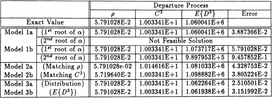
C

2 _E{D3

} Error

Exact Value 5.791028E-2 1.003341E+ 1 1.060041E+6

Modelia (I·t _{root of a) 5.791028E-2 1.003341E+1 1.060041E+6 3.887366E-2}

(2nd

root of a) Not Feasible Solution

Model 1b (16t _{root of a) 5.791028E-2 1.003341E+l 1.0737I7E+6 5.791028E-2}

(2n d _{root ofa) 5.791028E-2 1.003341E+l 9.897953E+5 9.457852E-l}

Model2a (Matching p) 5.791028e-02 1.014616E+1 1.081033E+6 4.328753E-2 Model2b (Matching C2

) 5.719640E-2 1.OO3341E+l 1.098882E+6 3.805224E-2

Model3a (Distribution) 5.791028E-2 1.OO3341E+l 1.062264E+6 2.510501E-2 Model3b

(E{D

3

} ) 5.791028E-2 1.003341E+l 1.061938E+6 3.151992E-2

Table 2: Arrival Process (PA = 0.931, qA= 0.99, llA = 0.458), a = 0.5, K

=

10

Departure Process

p 02 _E{D3

} Error

Exact Value 5.152882E-2 4.547770E+2 2.579378E+9

Modella

(l·

t root of a) 5.152882E-2 4.547770E+ 2 2.579377E+9 7.258830E-4

(2

nd

root of a) Not Feasible Solution

Modellb (l·t root of a) 5.152882E-2 4.547770E+2 2.579381E+9 7.203384E-4

(2

n d _{root of a)} Not Feasible Solution

Model2a (Matching

p)

5.I52882E-2 4.547778E+2 2.579386E+9 7.265276E-4 Model2b (Matching C2

) 5.152872E-2 4.547770E+2 2.579391E+9 7.257103E-4

Model3a (Distribution ) 5.152882E-2 4.547770E+2 2.579598E+9 5.619398E-4 Model3b

(E{D

3} ) 5.152882E-2 4.547770E+2 2.579378E+9 7.139101E-4

Depart ure Process

p

C

2 E{D3} Error

Exact Value 4.536092E-l 5.125532E-l 3.486905E+l

Model la (l"t root of Q) Not Feasible Solution

(2~d root of Q) Not Feasible Solution

Model l b (l"t root of Q) 4.536092E-l 5.125532E-l 3.520111E+l 2.368045E-2

(2

n-a root of Q) Not Feasible Solu tion

Model2a (Matching p) 4.536092E-l 5.798944E-l 3.970193E+l 5.798405E-2 Model2b (Matching C2

) 5.263209E-l 5.125532E-l 2.318192E+ 1 1.942099E-l

Model3a (Distribu tion) 4.536092E-l 5.125532E-l 3.518739E+l 2.160386E-2 Model3b (E{D3

} ) 4.536092E-l 5.125532E-l 3.518739E+ 1 2.143936E-2

Table 4: Arrival Process (PA == 0.38, qA == 0.35, aA == 0.9), a == 0.5, K

==

10

Departure Process

p

C

2 E{D3} Error

Exact Value 4.442376E-l 1.154362E+l 8.887376E+3

Model la (l"t root of Q) 4.442376E-l 1.154362E+l 8.843527E+3 2.988950E-3 (2n d _{root of Q) Not Feasible Solution}

Modellb (1"t root of 0) _{4.442376E-l 1.154362E+ 1} 8.920011E+3 1.432366E-3

(2n d _{root of a) Not Feasible Solution}

Model2a (Matching

p)

4.442376E-l 1.172159E+l 9.062557E+3 5.744578E-3 Model2b (Matching C2

) 4.368380E-l 1.154362E+l 9.230488E+3 1.416369E-2

Model3a (Distribution) 4.442376E-l 1.154362E+l 8.901693E+3 6.735641E-4 Model3b (E{D3

} ) 4.442376E-l 1.154362E+l 8.887359E+3 9.321133E-4

Table 5: Arrival Process (PA

==

0.99, qA

==

0.98, 0A

==

0.92), (J'

==

0.4, K

==

10

Departure Process

p C2 E{D3

} Error

Exact Value 4.343637E-l 4.667238E+2 7.821237E+6

Modella (l·t root of a) 4.343637E-l 4.667238E+2 7.821195E+6 5.623969E-4 (2nd _{root of a) Not Feasible Solution}

Model1b Il·t root of a) 4.343637E-l 4.667238E+2 7.821347E+6 5.344818E-4 (2nd _{root of a) Not Feasible Solution}

Model2a (Matching

p)

4.343637E-l 4.667373E+2 7.821572E+6 5.76030IE-4 Model2b (Matching C2) 4.343511E-l 4.667238E+2 7.821800E+6 5.362369E-4 Model3a (Distribu tion ) 4.343637E-l 4.667238E+2 7.822625E+6 3.000837E-4 Model3b (E{D3} ) 4.343637E-l 4.667238E+2 7.821239E+6 5.540679E-4

Depart ure Process

p

C

2 _E{D3

} Error

Exact Value _{8.946945E-l 1.051590E-l 1.998816E+0} Model la (l·t _{root of 0:)}

Not Feasible Solution

(2-n d _{root of0:)}

Not Feasible Solution Model Lb (l·t root of0:) _{Not Feasible Solution}

(2

n d

root of0:) _{Not Feasible Solution}

Model2a (Matching p) 8.946945E-l 1.053550E-l 2.000522E+O 3.068693E-4 Model2b (Matching C2

) 8.948905E-I 1.051590E-l _{1.998057E+0 6.164025E-4}

Model3a (Distribu tion) 8.946945E-l 1.051590E-l 1.998700E+0 1.837207E-5 Model3b (E{D3

} ) 8.946945E-l 1.051590E-l _{1.998700E+0 1.835226E-5}

Table 7: Arrival Process (PA == 0.9999, qA== 0.4999, 0A == 0.91), a == 0.1, K == 10

Departure Process

p

0

2 _E{D3

} Error

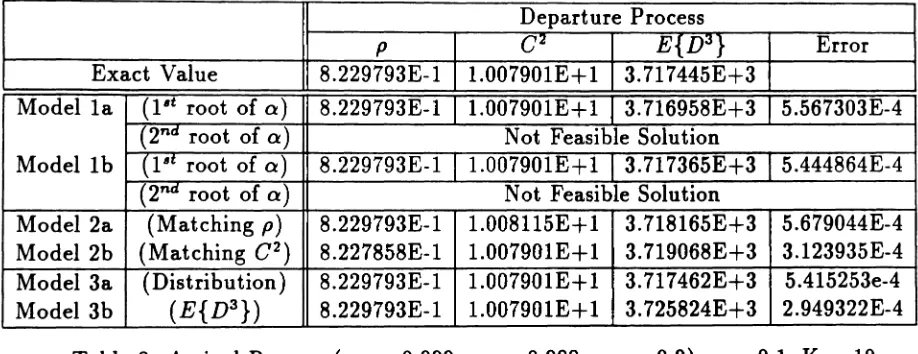
Exact Value 8.229793E-l 1.007901E+1 3.717445E+3

Model 1a (1·t _{root of a) 8.229793E-l 1.007901E+l 3.716958E+3 5.567303E-4}

(2n d

root of a) Not Feasible Solution

Model1b (l·t _{root of a) 8.229793E-l 1.007901E+l 3.717365E+3 5.444864E-4}

(2

nd _{root of Q) Not Feasible Solution}

Model2a (Matching p) 8.229793E-l 1.008115E+l 3.718165E+3 5.679044E-4 Model2b (Matching C2

) 8.227858E-1 1.007901E+1 3.719068E+3 3.123935E-4

Model3a (Distribution) 8.229793E-l 1.007901E+l 3.717462E+3 5.415253e-4 Model3b

(E{D

3

} ) 8.229793E-1 1.007901E+1 3.725824E+3 2.949322E-4

Table 8: Arrival Process (PA == 0.999, qA == 0.988, QA

=

0.9), a == 0.1, K

=

10

Departure Process

p

C

2 E{D3} Error

Exact Value 7.613183E-1 3.909688E+2 3.373541E+6

Modella (l·t _{root of a) 7.613183E-1 3.909688E+2 3.373439E+6} 1.013476E-5

(2

nd _{root of a) Not Feasible Solution}

Modellb (l·t root of

a)

7.613183E-l 3.909688E+2 3.373582E+6 3.755092E-5 {2nd _{root of}

a)

Not Feasible Solution

Model2a (Matching

p)

7.613183E-l 3.909993E+2 3.373846E+6 2.187076E-5 Model2b (Matching C2) 7.612587E-l 3.909688E+2 3.374110E+6 1.190766E-4

Model3a (Distribution) 7.613183E-l 3.909688E+2 3.373545E+6 5.881160E-7 Model3b

(E{D

3} ) 7.613183E-l 3.909688E+2 3.373545E+6 5.881123E-7

5

Analysis of a Tandem Configuration with Cell

Loss

In this section, we analyze approximately a tandem configuration of discrete-time finite

capacity queues using the fitting models described in the previous section. Let us consider

an open queueing network consisting of N nodes linked in tandem as shown in figure 4. The

nodes are numbered from 1 to N starting from the leftmost node. We assume that each node has a finite capacity. Let K, be the maximum capacity of node i, i

=

1,2, ... ,N. A

cell enters a node if it arrives at a time when the node is not full. Otherwise, it gets lost.

The arrival process to the first node is assumed to be an IBP. For eachnode i, the service

time is assumed to be geometrically distributed with probability O'i. We note that the N

servers are not synchronized. That is, the service slots of a server begin at a different time

than the service slots of the other servers. However, all service slots of all servers are equal.

Finally, we assume that cells in a node are served in a FIFO manner.

The approximation algorithm decomposes the queueing network into individual nodes,

and each node is analyzed in isolation. Let us consider node i. We can obtain the generating

function of the interdeparture time of node i using equation (11). Using one of the fitting models mentioned above, we can then obtain the set of parameters

{p,q,a}

of an IBP which

characterizes approximately the departure process of node i. This IBP becomes the arrival

process to the next down-stream node i

+

1. Since the arrival process to node i

+

1 is modeled as an IBP, node i

+

1 can also be analyzed as an IBP /Geo/l/Ki+1 queue. In the

examples given below, each queue is analyzed numerically using the Gaussian elimination

method. In this manner, we can analyze all queues individually starting from the first node and proceeding sequentially to the last node. A summary of the algorithm is given below.

step 0: Set i = 1.

step 1: Obtain the queue length distribution and the cell loss probability at node i.

Ifi

<

N, go to step 2. Else, stop.

step 2: Compute the generating function of the distribution of the interdeparture time of node i. From the generating function, calculate p, C2 _{and third moment.}

IBP

Figure 4: An open tandem queueing network under investigation

step 4: Set i

=

i

+

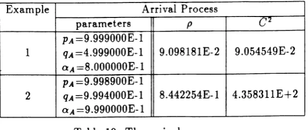
1 and go to step 1.

The accuracy of the approximation algorithm was tested by analyzing a 10 node ta.ndem

configuration. Two different examples were considered, one corresponding to a case of small

buffers and the other to a case of large buffers. The parameters of the arrival process to the

first node for the two examples are given in Table 10. The values of K, and lTi for example

1 are: Ki== 5 for i

==

1,3,4,7,8,9, Ki== 10 for i

=

2,5,6,10, lTi=0.1 for i

=

1,3,4,6,7,8,9,

and 0',:==0.2 for i

==

5,10. The values of K, and U'i for example 2 are: Ki= 32 and a,

=

0.1

for i

=

1,2,···,10. The approximation results were compared against simulation data in Figures 5-15. In particular, figures 5-10 are for example 1, and figures 11-15 for example 2.

The approximate results for example 1 were obtained using model 2a. (Model 3b was

also used but it gave identical results. The estimated squared coefficient of variation of the

interdeparture time, however, obtained using model 2a has 8. slightly larger relative error

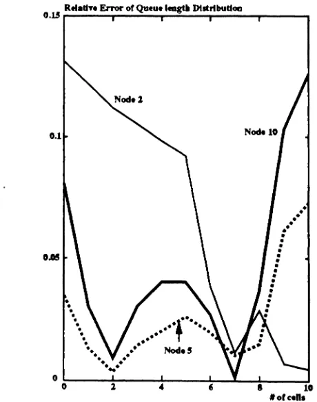
than that of model 3b.) In Figure 5 we give the queue length distribution for nodes 2, 5,

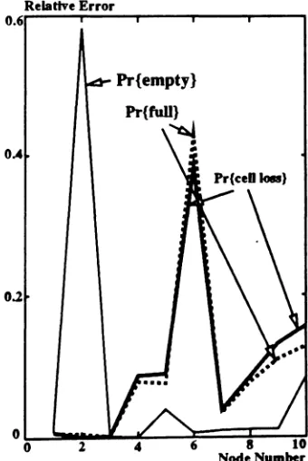
and 10. In Figure 7 we give the Pr{empty}, Pr{full}, and cell loss for each queue. The cell

loss probability at a node is

Pr{Node is full

I

an arrival occurs}

=

_KP(O, K)(l - qA)aA

+

P(l,K)PACtA

L[P(O,n)(l - qA)aA

+

P(l,n)PAoA]

n=O

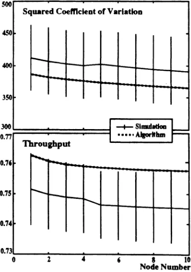
Finally, in Figure 9 we give the throughput and squared coefficient of variation of the

inter-departure time for each node. Relative errors are given in Figures 6, 8, and 10. We note

that the confidence intervals were not plotted as they were extremely small. Also, the large

Example Arrival Process

parameters p

C

2

PA=9.999000E-l

1 qA=4.999000E-l 9.098181E-2 9.054549E-2

0A=8.000000E-l

PA=9.998900E-l

2 qA =9.994000E-l 8.442254E-I 4.35831IE+2

0A=9.990000E-I

Table 10: The arrival processes

are extremely smallIi.e. less than 10-3 ) .

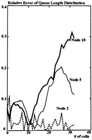
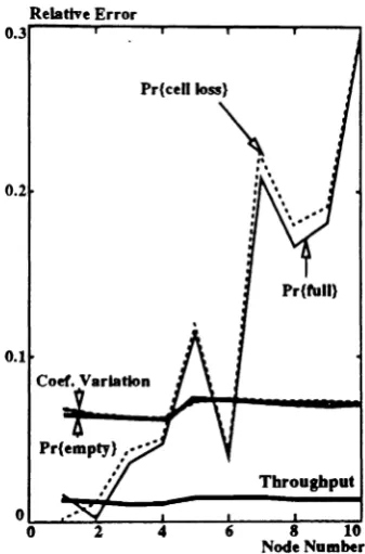
The approximate results for example 2 are given in Figures 11- 15. These results are

presented in the same way as in example 1. Model 28., 3b, and a combination of models la

and 2a were used. Models La and 2a were combined as follows: use model la if it gives a

feasible solution. If the solution is not feasible, then use model 2&. The results obtained

using these fitting models are identical. (The estimated squared coefficient of variation of

the interdeparture time was the same for all models.) In view of this, we are only present

the results obtained using model 2a.

In general, all fitting models give about the same accuracy. Model 3 gives the best

esti-mate for the distribution of the interdeparture time of each queue but it is time consuming.

The other models, such as model 2a or the combined models la and 28., can give better

estimates for the queue-length distribution or the cell loss probability. As mentioned earlier,

model 2a gives estimates of the squared coefficient of variation of the interdeparture time that

has a larger relative error than those obtained using other models. The combined method

of model laand 2& seems to provide the best approach as it has a satisfactory accuracy and

6

Conclusion

In this paper, we proposed various models for characterizing the in terdepart ure time of a

discrete-time IBP /Geo/l/K queue by an IBP. We applied these models to analyze a tandem

Queue Length Dtatribudon

0..5~---..,..---...----r---""'T"----'

0.4

-+-Simulation ••• Alaortthm

0.2

0.1

Figure 5: Queue length distribution (example 1)

R".U~.Error ofQueueIeagtIIDllItrtbutioo

0.15 ....- - - . ...- - - - . - - - -...- - -...- - -..

0.05

10 'olcen.

ProbablUty

O.IS

Pr{empty}

Pr{ceU loss}

O_ _-..._ _....r..- ~ _ ~ _ . _ _ .

o

0.1

O.M

Figure 7: Pr{ empty}, Pr{full}, and Pr{ cell loss} (example 1)

Relative Error 0.6

4

Pr{empty}

Pr{full}

~_•

-oL~_o ...L.L.-~==;=~

0.2 OA

0.8 Throughput

0.6

-+- Simulation •••• Algortthm

0.4

Squared Coef. Variation 0.1

6 8 10

Node Number 4

2

O"",,"-_~_ _... ~_--....

o

Figure 9: Throughput and squared coefficient of variation (example 1)

RelatmError

O.n"tr---...---y---r---...----.

O.OIS

0.01

o.OOS

Throaghput

...

••••

•...

...

.

4 6 8 10

Node Number

0.2,..Q_ueue_ _Len...at_h.,.D_I8tr_ Ibu_ tlQ_n---r r - - _

O.IS

-+-SI.uI.tlon ••• AJaorfthlll

0.1

O.OS

o

, ofcelli

Figure 11: Queue Length Distribution (example 2)

Relative Error of Queue Length Dktrlbutton

0.4

ProbabDHy

0.2

0.1~ Pr{empty)

0.1 Pr{ctO10M}

Pr(faB)

0.05

~S"'aI.tIoD

•••• AJIO"Ulam

6 8 10

Node Number

Figure 13: Pr{ernpty}, Pr{full}, and Pr{cellioss} (example 2)

soo

Squared CoemcleDt of VartatloD

4SO

400

350

.

Throughput

...

~­

I""~~~~

...

.J

300

r

-+-Sh..d8doa

0.77=======:::::::::=::::1

1 •••••AJaorIthm

0.75

0.74

2 4

,

8 10

Node Number

Relative Error 0.3

0.2

Pr{tull}

0.1

4

Throughput

6 8 10

Node Number

A

Appendix

Given a value of 0, where 0

<

a ~ 1, we can obtain the following solution for p and q (see section 4.3).

p

q

(02

- 1)a

+

3ap - 2p2

(C2 - l)« - ap

+

2a2

'

(C2 _{- 1)a - 3ap}

+

_2a2

+

_2p 2

(C2 - 1)a - ap

+

2a2

(23)

(24)

we show that if conditions (1) to (3) hold then 0 <p< 1and 0 < q < 1.

(a) If(C2 _-l)a

+

_{3ap - 2p}

2 >0 then 0

<

p < 1.

proof:

Since the following relation

is always true, we have that the relation,

2(0: - p)2

>

0

(02

- 1)0: - ap

+

20.2

>

(02 - 1)0:

+

30.p - 2p2

>

0

is also always true if (C2 _{- l)a}

+

_{30:p - 2p2 >0. Since the numerator and denominator in}

equation (23) are all positive and the denominator is larger than the nominator, we have

that 0

<

P

<

1.

(b) If(C2

- 1)0. - 30:p

+

2p2

+

20.2 >0 and and p

<

a ~ 1 then 0

<

q

<

1.

proof:

If can be easily shown that following relation

is true if p

<

a. Hence, if p

<

a and (02

REFERENCES

[1] A. Bhargava, J. Kurose, D. Towsley, and G. Vanleemput. Performance comparison of error control schemes in high-speed computer communication network. IEEE J. Select.

Areas Commun., (9), Dec. 1988.

[2]

P. P. Bocharov and

F. K.

Albores. On two-stage exponential queueing system with internal losses or blocking. Probe Control Inform. Theory, 1980.

[3] J. Hsu and P. Burke. Behavior of tandem buffers with geometric input and Markovian output. IEEE Trans. Commun., Mar. 1976.

[4]

H. Kobayashi, Modeling and Analysis: An introduction to system performance evalua-tion methodology. Reading, MA: Addison- Wesley Publishing Company, 1978.

[5] T. D.

Morris and

H. G.

Perros. Performance analysis of a multi-buffered Banyan

ATM

switch under bursty traffic. to be presented in INFOCOM '91.

[6] J. Morrison. Two discrete-time queues in tandem, IEEE Trans. Commun., (3):563-573,

Mar. 1979.

[7] A. Nilsson, F. Lai, and H. G. Perros. An approximate analysis of a bufferless NxN synchronous class ATM switch. In Queueing Performance and Control in AT~[. Cohen, and Pack, Eds. North Holland, 1991.

[8] Y.

Ohba,

M.

Murata, and

H.

Miyahara. Analysis of interdeparture process for bursty traffic in ATM networks. IEEE J. Select. Areas Commun., (3), Apr. 1991.

[9]

G. Pujolle. Multiclass distrete-time queueing systems with a product form solution.

Int'l. Seminar on the Performance of Distributed and Parallel Systems, Sept. 1991.

[10]

G. Pujolle and H. G. Perros. Queueing systems for modelling ATM networks. Proc.

of the Int'l. Conf. on the Performance of Distributed SY6tems and Integrated Comma Networks, Kyoto, Sept. 1991.

[11]

P. Tran-Gia. Discrete time analysis for the interdeparture distribution of GI/G/1 queue. In TeletraJfic Analyl" and Computer Performance Evaluation, pages 341-357. O. J.