Assessing the effects of measurement errors in line transect sampling

•

n

Mrt,men\

0'

StatistiCS

The l\btafY

of

\be

vet'" "

C

<

\'oa State

UmvefS1t'J

North am'

< :

Assessing the effects of measurement errors in line

transect sampling

Russell Alpizar-Jara, L. A. Stefanski,

K. H. Pollock, and J.L. Laake*

Department of Statistics

North Carolina State University

Box

8203,

Raleigh, NC

27695-8203

National Marine Mammal Laboratory*

Alaska Fisheries Science Center

NMFS,

7600

Sand Point Way N.E.

Seattle, WA

98115

Institute of Statistics

11imeograph Series No.

2508

North Carolina State University

Raleigh, North Carolina

"

Abstract

We evaluate the effects of measurement error in population parameter estimation from a line transect sampling model,. characterize the error. distribution, and illustrate . using data from a controlled field experiment (Stakes data set, Laake 1978). We de-scribe a methodology to estimate the measurement error variance from a replicated experiment assuming an additive measurement error model, and correct for system-atic measurement error bias in the population estimates using calibration (Carroll et al. 1995). A simulation based method of inference for parametric measurement er-ror models is suggested to correct for random effects measurement erer-ror biases (Cook and Stefanski 1994). A simulation study is conducted to show the potential effects of measurement error in a line transect studies. Two main sources of measurement error biases were found in the stake data set, systematic and random effects. In this particular study, the systematic measurement error bias causes overestimation, and the random effects measurement error biases cause underestimation of population size and density. The random effects biases were not as severe as the systematic bias.

KEY WORDS: Calibration, line transect, SIMEX, systematic and random measure-ment error, wildlife density estimation.

.1

Introduction

One of the fundamental assumptions of line transect sampling is that distances from the transect line are measured without error (Buckland

et aI.,

1993). Enough evidence exists in the literature to show that measurement errors have an important effect on the estimates of population size, N, and density D. However, sound approaches to quantify and account for this effect in population estimates have not received enough attention.

problem of measurement errors using some data from Robinette et al. (1974). Their analysis suggests that considerable measurement and rounding errors occurred near the transect line. Buckland et al. (1993, p.317) include a section on measurements and emphasize the importance of collecting accurate measurements in distance sampling, and someimplicati~ns of errors in the measurements. The authors mention several reasons to support the use of perpendicular rather than radial distance models, and discuss possible solutions to cope with measurement errors in distance sampling data. Buckland and Anganuzzi (1988) proposed an

ad hocmethod of estimating the smearing parameters, and compared their method with other existing methods. "Smearing" is a method that has been often used to analyzed cetacean shipboard surveys where sighting distance and angle data are more likely to be collected. The concept of smearing was first introduced by Butterworth (1982). For a description of this method see Buckland et al. (1993, p. 319).

Borchers and Haw (1990) pointed out the need for more accurate estimation methods when analyzing data based on radial distances (sighting distances and angles) rather than perpendicular distances. They conducted experiments on Antarctic sighting surveys and identified several sources of biases and imprecision in the measurements. Schweder et al. (1991) attempted to estimate error and bias in radial measurements based on triangulated data from the parallel ship experiments. 0ien and Schweder (1992) obtained estimates of bias and variability in visual distance measurements made by observers.

Recently, a more formal treatment to the problem of measurement error in line transect surveys has been addressed by Chen (1997). Chen proposes a method of moments estimator to correct for measurement error induced bias, and assumes an exponential power series detection function. He also assumes up to a fourth moment of the error distribution, and his method requires knowledge of the side of the transect on which an observation has been collected (i.e. signed perpendicular distances).

by Carroll et al. (1995). The next section introduces the basic line transect model and some notation. Section three introduces key concepts of measurement error models as they apply to a line transect sampling study with measurement error. Section four describes a controlled line transect study which is used to illustrate the methods suggested in this paper (Stake data set, Laake 1978). Section five characterizes the distribution for the stake data set using some exploratory data analysis techniques. An additive measurement error model and measurement error variance estimation is discussed in section six. Bias correction using calibration and SIMEX is discussed in section seven. Finally, a discussion and future research directions in section eight concludes.

2

Basic line transect model

A brief description of this model is given here. See Buckland et al. (1993) for a good detailed exposition on theory and applications.

Line transect sampling consists of defining straight lines across an area of known bound-aries. Observers travel along the lines (walking, riding on horseback, on a ship, on an airplane, etc.) detecting a sample of target objects, and recording at the moment of detec-tion the perpendicular distance from the line to a detected object, or the sighting distance from the observer and the angle between the line of travel and the line of sight to the ob-ject. Ifpossible perpendicular distances are measured, but if not then the sighting distance and angle are usually converted to perpendicular distance by a trigonometric relation (i.e. perpendicular distance equals sighting distance times sine of the sighting angle) (Buckland et al. 1993).

2.1

Assumptions

The basic assumptions underlying the line transect sampling model are:

(i)

Objects directly on the line have probability one of being detected.

(iii)

The measurements of distances and angles are exact (i.e. there are no measurement

errors or rounding errors).

(iv)

The sighting of one animal is independent of the sighting·of another.

These assumptions can easily be violated according to the particular practical conditions

of each study. The validity of the model will depend on there being little violation of the

assumptions; therefore, the design of the study should attempt to minimize all possible

violations. This paper focus on issues related to assumption

(iii).

This assumption is

violated if measurements are only roughly estimated. Extensive work have been done to

relax the other assumptions, but little have been done on measurement errors. See Buckland

et al. (1993) for a detailed discussion of assumption violations.

2.2

Notation

Nw is the population size in the surveyed area.

L is the total line length in a line transect survey.

w is the half-width of a strip transect of L length.

Aw

=

2wL is the surveyed area.

i

=

1, ,Nw is used to index the observations (i.e. objects, animals).

j

=

1, ,]{ is used to index the replicates (i.e observers in the stakes study).

ki is the number of replicates in which observation i is detected.

nj is the number of observations (sample size) detected in replicatej.

Xi

are the exact perpendicular sighting distances.

Wij are the observed perpendicular sighting distances measured with error.

Uij are the errors associated to the measurements.

ft

is the vector parameter describing the detection function.

g( .

1ft)

is the detection function.

f( .

1ft)

is the probability density function of perpendicular distances.

(1)

to be detected. Objects that are far away from the transect center line usually have lower probability of being detected than those closer to the transect center line. Modeling this drop in detection probability is central to line transect sampling. This drop is modeled with a decreasing function relating the probability of detecting an animal and its perpendicular distance from the line. This function is known as the detection or sighting function,

g(X

i ),

which properly scaled can be used as a probability density function,

!(Xi).

Thus, population and density estimates are directly dependent on accurate measurement of the distances because

g(Xi)

needs to be estimated from the available distance information. Ifdistances are measured inaccurately, the estimate of the detection function will be biased. It can be shown that if the above assumptions, in particular assumption (i), are satisfied then the estimators of density and population size are given by

b

=

N

w

=

_nj(O)

Aw 2L

where

N

w is an estimator of the total population in the area covered, Aw

=

2wL. L is

the total length of the transect strips of width w. It is extremely important to randomly locate lines in the area; otherwise, is necessary to assume that objects are randomly and independently distributed over the population area which in many cases it is an unreasonable assumption. Also, it is recommended that several random lines be used so that robust variances of estimates can easily be obtained.

In equation (1), note that the key parameter to estimate is

!(O),

the probability density function evaluated at distance zero. This parameter is directly proportional to the population size estimator

N

w = nwj(O), and if distances near the line are measured with error, the

estimators of Nand D are biased.

3

Measurement error models

mea-surement error in linear models, and more recently Carroll et al. (1995) on meamea-surement error in nonlinear models. In the remainder of this paper, some of the key concepts of mea-surement error models as they apply to a line transect sampling study with meamea-surement errors are introduced. The effect of measurement errors on the estimators of density and population size is assessed.

The discussion is based on the existence of an exact predictor X and measurement error models which provide information about this predictor. Our exact predictor is the per-pendicular distance measured without error, sometimes also referred as "true" or "exact" distance.

In line transect surveys, we are interested in modeling the probability density function,

f(XI!l), as a function of the exact perpendicular distance, the predictor X. In practice, X

can not be observed exactly for all individuals in the study. However, we can observe a variable W (Le. observed perpendicular distance) which is related to X. The parametric modelf(XI!l) can not be estimated directly by fittingJ(·lfD toX. SubstitutingW forX, but making no adjustments in the usual fitting methods (i.e. maximum likelihood or nonlinear least squares) for this substitution, leads to estimates that are biased, sometimes seriously (Carroll et al. 1995). The goal of using measurement error modeling is to obtain nearly unbiased estimates of!l.

4

A controlled field study: the stake data set

Laake (1978) conducted an investigation of line transect sampling by placing a known number of wooden stakes in a rectangular area of sagebrush meadow east of Logan, Utah. The stakes were randomly placed and uniformly distributed as a function of distance from the line. Eleven independent observers walked along a transect line of length L

=

1000 meters and a fixed half- width strip of w

=

20 meters.

The stake data is a very well known data set that has been analyzed on several occasions. Burnham

et ai.

(1980) analyzed this data set and found that the number of observed stakes varied substantially among observers, and that the underlying detection functions

g(X)

differed greatly among observers. The data provided an estimate of the average density of 31.6 stakes per ha., but the true density was 37.5. Burnham

et

al. (1981) considered that this negative bias is at least partially due to the failure of the assumption that all stakes on the centerline were detected. Buckland

et ai.

(1993) have done some additional analyses and found that some of the negative biases in the population estimates are due to measurement error for stakes near the line. Measurement errors in the stake data could also be related to heaping and rounding effects when observers estimate distances from the centerline.

For the stake data set, the exact location of each stake was known, and also the estimated distances for the stakes seen by each of the eleven observers are available. Itis possible to identify which stakes were seen by each observer, and an estimate of the measurement error variance can be obtained as we shall show. Another advantage of using the stake data set is that the population size is known (N

=

150 stakes), hence our population estimates can be compared to the true population parameter. Also, it is an immobile population, and thus we do not have to worry about violation of the assumption that objects do not move before being detected,

(ii),

which also introduces an effect in the measurement of the distances.

of the measurement error variance. In this study, each observer's estimated distance to a detected stake was considered to be a replicate measurement of the distance to that stake.

5

Characterization of the error distribution

To evaluate the effect of measurement errors in the stake data set, an exploratory data analy-sis was carried out using the distances measured by the eleven observers. Often, measurement errors are assumed to be normally distributed to simplify analysis and the construction of confidence intervals for population parameters. The error distribution is first characterized instead of blindly assuming normality.

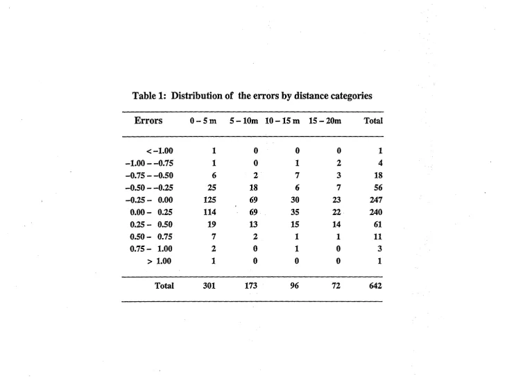
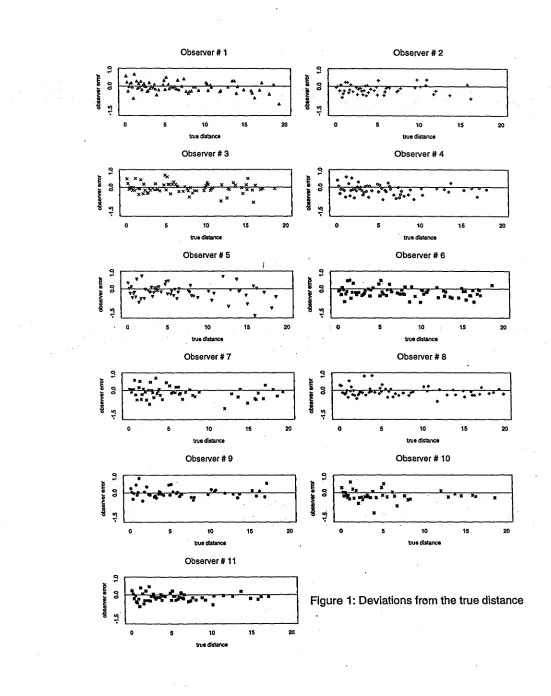
Figure 1 displays the observers errors vs. the "true" distances. Important features of this line transect study can be obtained from examining this plot. Notice for instance that there is a concentration of points near to zero distance, and sometimes a few points far away from the line. There is a clear drop in the sightings as distance increases. Itis also possible to appreciate the magnitude and direction of the error. Sometimes errors were as large as one meter or more, and there is a slight tendency to underestimate the true distance. Table 1 summarizes the distribution of the errors by distance categories.

[Table 1 and Figure 1 near here]

[Figures 2a,b near here]

6

The

effects of measurement error and estimation of

measurement error variance

A simple univariate additive error model is considered, where conditional on X, the errors have mean zero and constant variance, O"~. For a single observation, assume the model

Wij

= {3o

+

{3xXi

+

Uij

with

Uij

rv (0,O"~).

For each stakei that was detected by at least one observer, we compute the average of the observed distances given that a stake was located at true distance

Xi

(fixed by design). It is reasonable to assume that ifthere is no effect of measurement errors, the plot of the average of the observed distances

(Wd

versus the true distances

(Xi)

should fall on a straight line with slope one and intercept zero. We then hypothesize the following model for the average of observed distances,

(2)

where

2

Note also that

E(Wi.\Xi)

=

(30+{3xXi,

and

Var(Wi.IXi)

=

~;,

where

O"~

is the measurement error variance for a single observation.

To find out ifthere is any systematic measurement error bias the following hypotheses need to be tested,

Ho : {3x

=

1

and

Ho :

(3o

=

o.

the distances. Determining the magnitude and direction of this effect is also of interest. If

H

o :

f30

= 0 is rejected, then this indicates that measurement errors have a strong effect on

distance measurements close to line (at zero distance).

Since an observation depends on whether a stake was detected or not, the number of

replicates for each stake is not fixed. Observations do not contribute equally to the fit.

We use weighted least squares (Draper and Smith, 1981) to estimate the parameters of this

model. After fitting the model, the data can be calibrated by adjusting the observed averages

to obtain the additive error model

(3)

where

~w.

= Wi. -

,80

~U.

- U

i.

and

~U

N (

a~)

(4)

t·

,8x'

t' -

,8x

i· '" 0,

,8; .

Under these model assumptions, an estimate of the measurement error variance after

cali-bration is given by

A2

A2 au ( )

aU"

=

- A , 5

f3-;

which is estimated dividing the mean squared error of the fitted weighted regression model

by the the estimate of the slope.

To determine whether there is some degree of heteroscedasticity in the measurement error

variance given the "true" distance, one could hypothesize that the variance of the observed

distances would increase for observations further away from the transect line. The following

could be used as a baseline model,

(6)

1 k·

2 ~ - 2

Si

=

k. _ 1?---(W

ij -

Wd ,

, 3=1

and then fit the model using least squares weighting by the number of observations in which 2 each

Sl

is based (i.e. k

i -

1). Note that

E(SlIXi)

=

10

+

lxXi,

and

Var(SlIXi)

=

~.

ki - 1

We are interested in testing the following hypothesis,

Ho : IX = 0

IfHo :IX = 0 is rejected then the variance of the observed measurements given the true distance increases linearly as true distance increases. IfIX = 0, then constant variance should be assumed and an additive model is appropriate. Also, an estimate of the measurement error variance for a single observation is given by the estimate of the intercept

(10)

since

E(SlIXi)

=

10.

Results from the fitted models,

Wi.

=

fJO+fJxXi

and

Sf

=

10 +1xXi,

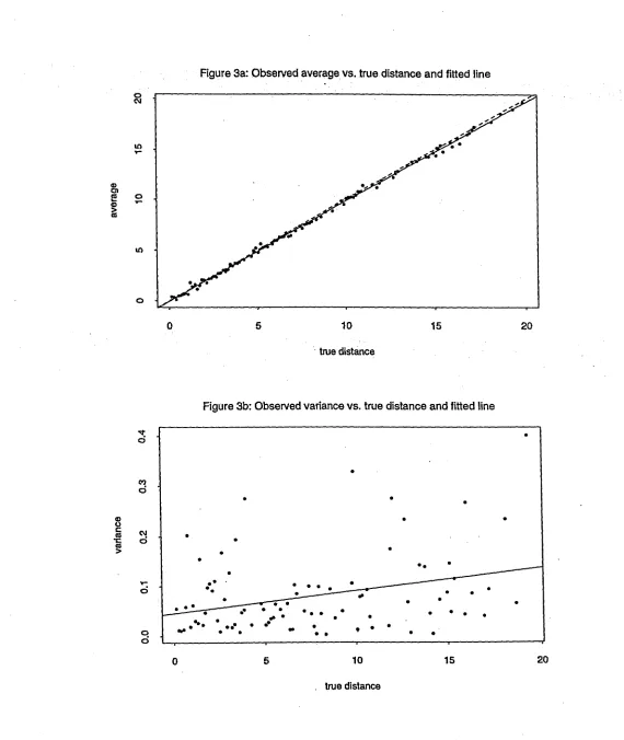
using the stake data set are given in Table 2. We used SAS procedure REG (SAS Users Guide) for the analysis. Plots corresponding to these fits are given in Figure 3.

[Table 2 and Figures 3a,b near here]

The null hypothesis H_{o :} f3x = 1 is rejected in favor of the alternative H_{o :} f3x

<

1.

A

f3x = 0.989, with standard error 0.004. This result indicates that there is a systematic effect of the measurement errors in the measures of perpendicular distances. Observers tend to underestimate the true perpendicular distance. This result is also confirmed by the exploratory data analysis form the previous section (Figure

1),

in which generally more than half of the observations detected by each observer are below the zero line. An estimate of the measurement error variance of the calibrated measurements is given by

~;

=

0.2826

=

0.2888.

Although we reject the null hypothesis H_{o :} IX

=

0,

(p

=

0.0154), the model does not give a good fit to the data

(r

2

=

0.067) (Figure 3). Also, the exploratory data analysis does not suggest strong evidence of heteroscedasticity for this model (Figure 2).

In assessing the measurement error effects we also fitted several parametric models to the data collected by each observer. Models were fitted to both, "true" and observed per-pendicular distances. Program DISTANCE (Laake et al. 1993) was used for model fitting using maximum likelihood estimation, and model selection was carried out using the Akaike Information Criteria (Akaike 1973). Models that "best" fitted the data with the correspond-ing population estimates are shown in Table 3. Note that in most cases a half-normal model was selected as the "best" fit, and in some occasions a uniform detection function with up to three cosine adjustment terms (see models for Observer 6).

[Table 3 near here]

These results suggest that there may be some effects of measurement errors in model selection. For instance, for Observer 1 a uniform model with one adjustment cosine term was selected when fitting the model with the true distances, but a half-normal model with no adjustment terms was selected when using the observed distances. Also, note that in most cases the true population size N = 150 is underestimated although the true value is generally contained in the confidence intervals. Possibly, this negative bias is largely due to violation of the assumption that stakes on the centerline have probability one of being observed rather than to the effect of measurement errors.

distances were consistently underestimated. To correct for this systematic bias, calibration

of the data is required.

7

Bias correction using calibration and SIMEX

In this section we use some stake data and simulations to illustrate bias correction using

calibration to account for the systematic measurement error effects, and to demonstrate

the random measurement error effects on population size. We also describe and suggest

the SIMEX algorithm (Cook and Stefanski, 1994) to correct for bias due to the random

component.

For the sake of illustration the data collected by Observer 4 has been chosen, and fitted a

half-normal model with no adjustment terms for the true and observed distances. The

max-imum likelihood estimates of population size and their standard errors obtained from these

fits are

N

w

=

122(19.3) and

N

w

=

125(19.6) for the true and observed distances respectively.

As noticed from the data analyses for all the observers in the preceding section,

overesti-mation is caused by the tendency of each observer to underestimate the true perpendicular

distances. Observer 4 was not an exception. We calibrate the observed data as described

earlier, (see equation 4 in previous section), to reduce this systematic bias. After calibration

of the observed distances, we fitted the same model and obtained an estimate of population

size of

N

w

=

123(19.3). Note that this population estimate is now closer to the error-free

population estimate and we have corrected for some of this systematic effect.

The simulations to be described are based on the SIMEX algorithm. SIMEX is a

simulation-based method of inference for parametric measurement error models to adjust

for the random effects of measurement error bias (Cook and Stefanski 1994, and Stefanski

and Cook 1995). The authors show that the magnitude of this random effect bias in the

estimates depends on the size of the measurement error variance. The simulation step of

SIMEX is used to examine the effect of the random component. The method requires that

set the random measurement error effects are not large enough, we do not use the extrap-olation step of the SIMEX algorithm to correct for this effect. If the effects of random measurement errors were large, we suggest using the full SIMEX algorithm to correct for bias due to the random component.

Cook and Stefanski (1994) developed a simulation-based estimation procedure for mea-surement error models known as SIMEX (Simulation-Extrapolation). The SIMEX method has been shown to produce less biased parameter estimates. The main idea using SIMEX is to experimentally determine the random effect of measurement errors on an estimator via simulation. Ifan estimator is influenced by random measurement errors, simulation exper-iments can be considered in which the level of the measurement error, (i.e. its variance), is intentionally varied (Carroll et al. 1995, p.80). SIMEX estimates are obtained by adding additional measurement error-induced bias versus the variance of the added measurement error, and extrapolating this trend back to the case of no measurement error. In synthesis, the SIMEX algorithm consists of four main steps:

(i)

Additional measurement error is added in known increments to the observed data.

(ii)

For each increment of added measurement error, parameter estimates are computed from the further-contaminated data.

(iii)

A trend is established between the parameter estimate and the added measurement error. (iv) The trend is extrapolated back to the case where there is no measurement error. Details on the theoretical support of the SIMEX estimate can be found in Stefanski and Cook (1995). SIMEX is best suited to problems with additive measurement error models, but additivity of errors is not crucial and the method can be extended to more general models (Carroll et al. 1995). Although the focus in this paper has been an additive measurement error model, additional analyses have been done assuming a multiplicative error model. For reasons of space, these analyses are not presented here.

of the half-normal detection probability density function,

/('10).

In the simulation step we create additional data sets of increasingly larger measurement error (1

+

>,)(J~,

>.

=

{O.O,

0.25, 0.50, ... , 2.0}. The measurement error variance estimate obtained in the previous

section, given by (5) was used as an estimate of(J~. For any

>.

~ 0, we define

Wb,i

=

Wi

+

..r>.Ub,i,

i = 1, ... ,n,

b

= 1, ... ,

B,

(7)

where the computer-generated pseudo-errors,

{Ub,i}i=l'

are mutually independent, indepen-dent of all the observed data, and iindepen-dentically distributed normal random variables with mean zero and variance (J~. Once the new predictors are created, the average of the estimates ob-tained from a large number of experiments, (B

=

500 in our study), with the same amount of measurement error are computed and plotted versus the amount of error added

(>.).

The estimated value at

>.

= 0 (i.e. no measurement error added to the contaminated data) is known as the the NAIVE estimator. The extrapolation step consists of modeling these av-erages as a function of

>.,

for .>.

>

0, and extrapolating the fitted models back to

>.

=

-1. The extrapolated value at

>.

=

-1 corresponds to the SIMEX estimator.

A simulation study was carried out in which known amount of measurement error can be added to error-free line transect data (i.e. true perpendicular distances) to determine the effects of random measurement error in the parameter estimates. If we were to do the extrapolation step, it would not make sense to extrapolate for the true distance data because the SIMEX and the NAIVE estimators are equivalent since the data are known to be error-free. The SIMEX simulation step was used to compare population estimates obtained from fitting the true, observed and calibrated perpendicular distances while adding known amounts of random measurement errors.

When fitting the calibrated perpendicular distances, we account for heteroscedasticity of the measurement error variance by modeling it as a function of distance as described in the previous section (see equation 6). Pseudo-data sets are generated using an estimate of the

t . . b A

2

1'0

+

1'x

X

i

measuremen error varIance gIVen y (Ju = A •

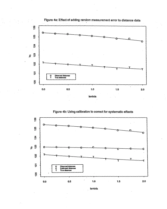
Results from these simulations are summarized in Figure 4. The solid line corresponds to fits of a quadratic extrapolant function. Clearly, adding more random measurement error to distance data causes underestimation of the population size estimates. The same declining trend is observed for analyses of the observed and true perpendicular distance data. Note however, that the random effect of measurement errors in the population estimates is minimal since the lines are almost flat curves (Figure 4a). Also note that the calibrated data produce estimates that are closer to those estimates obtained from the true distances even after adding large amounts of random measurement error (Figure 4b). This result suggests that a combination of calibration and SIMEX analysis removes of most of the measurement error.

[Figures 4a,b near here]

8

Discussion and future research

In this paper, the stake data set was used to obtain an estimate of the measurement error variance. The stake data set also allows characterization of the error distribution. Several advantages of using the stake data set are that the true distances at which the stakes were placed are known, and there were eleven observers walking along the line which allows reasonable estimation of the measurement error variance. The true population size is also known. Two main sources of measurement error biases were identified and quantified for this study, systematic and random measurement errors. Calibration was used to correct for systematic measurement error bias, and the simulation step of the SIMEX algorithm to examine the effects of random measurement error bias. For simplicity, a univariate model for the detection function (half-normal) is considered to illustrate the estimation methods. In synthesis, this paper suggests a general but simple methodology to assess the effect of measurement errors in line transect surveys, and to correct for measurement error bias.

in model selection using Akaike information criteria and maximum likelihood ratio tests also needs to be assessed. The robustness of estimation methods (Le. maximum likelihood esti-mation, nonlinear least squares, kernel density estiesti-mation, etc.) to measurement errors can be evaluated. Violation of the assumption of constant variance and the use of an alternative multiplicative model need to be investigated since the measurement error variance may be a nonlinear function of the distances (i.e. quadratic or exponential function). Some analyses in this direction have been done, but because strong evidence of heteroscedasticity was not found, and for reasons of space they are not included here.

References

Akaike, H. (1973) Information theory and an extension of the maximum principle. In

International Symposium on Information Theory, 2nd edn(edsB. N. Petran and F. Csaaki),

Akadeemiai Kiadi, Budapest, Hungary, pp. 267-81.

Borchers, D. L. and M. D. Haw. (1990). Determination of minke whale response to a

transiting survey vessel from visual tracking of sightings. Report of the International Whaling

Commission, 40, 257-69.

Buckland, S.T., D.R. Anderson, K.P. Burnham, and J.L. Laake. (1993) Distance

sam-pling: Estimating abundance of biological populations. Chapman and Hall, London. 446pp.

Buckland, S. T. and A. A. Anganuzzi. (1988). Comparison of smearing methods in the

analysis of Minke sighting data from IWC /IDCR Antarctic cruises. Report of the

Interna-tional Whaling Commission, 38, 257-63.

Burnham, K.P., D.R. Anderson, and J.L. Laake. (1980). Estimation of density from line

transect sampling of biological populations. Wildlife Monographs, 72, 202 pp.

Carroll R.J. and L.A. Stefanski. (1990). Approximate quasi-likelihood estimation in

models with surrogate predictors. Journal of the American Statistical Association., Theory

and Methods. 85(411), 652-663.

Carroll R.J., D. Ruppert, and L.A. Stefanski. (1995). Measurement errors in nonlinear

models. Monographs on statistics and applied probability 63. Chapman and Hall, London.

305pp.

Char, B.W et al. (1991) Maple

V

Library reference manual. Waterloo Maple Software.

Springer-Verlag, New York.

Chen, S.

X.

(1997). Measurement errors in line transect surveys. Technical paper

sub-mitted for publication to Biometrics.

Cook, J.R. and L.A. Stefanski. (1994). Simulation-extrapolation estimation in

paramet-ric measurement error models. Journal of the Ameparamet-rican Statistical Association., Theory and

'.

Draper, N. R. and H. Smith (1981). Applied regression analysis. John Wiley and Sons,

New York, New York, U.S.A.

Laake, J. L. (1978) Line transect estimators robust to animal movement, MS Thesis,

Utah State University, Logan, UT, USA, 55pp.

Laake, J. L., Buckland, S. T., Anderson, D.R. and Burnham, K. P. (1993) DISTANCE

User's Guide. Colorado Cooperative Fish and Wildlife Research Unit, Colorado State

Uni-versity, Fort Collins, CO 80523, USA.

MathSoft, Inc. (1995). S-PLUS Guide to Statistical and Mathematical Analysis. Version

3.3 for Windows and Unix. Seattle, WA. U.S.A.

0ien, N. and T. Schweder. (1992). Estimates of bias and variability in visual distance

measurements made by observers during shipboard surveys of northeastern atlantic minke

whales. Report of the International Whaling Commission, 42, 407-412.

Robinette, W. L., Loveless, C. M. and Jones, D. A. (1974). Field tests of strip census

methods. Journal of Wildlife Management, 38, 81-96.

SAS Institute Inc., (1990). SAS/STAT User's Guide, Version 6, Fourth Edition, Volume

2. Cary, North Carolina, 846 p.

Schweder, T. (1977). Point process models for line transect experiments, in Recent

De-velopments in Statistics (eds). J.R. Barba, F. Brodeau, G. Romier and B. Van Cutsem),

North-Holland Publishing Company, New York, USA, pp. 221-42.

Schweder, T., G. H~st, and N. 0ien. (1991). Estimates of the detection probability for

shipboard surveys of Northeastern Atlantic Minke whales, based on a parallel ship

experi-ment. Report of the International Whaling Commission, 41, 417-432.

Stefanski, L. A. (1985). The effects of measurement error on parameter estimation.

Biometrika 72(3):583-92.

Stefanski, L. A. and Cook, J. R. (1995). Simulation-Extrapolation: The measurement

Table 1: Distribution of the errors by distance categories

Errors

0- 5 m 5 - 10m 10 - 15 m 15 - 20m

Total

<-1.00 1 0 0 0 1

-1.00 - -0.75 1 0 1 2 4

-0.75 - -0.50 6 2 7 3 18

-0.50 - -0.25 25 18 6 7 56

-0.25 - 0.00 125 69 30 23 247

0.00 - 0.25 114 69 35 22 240

0.25 - 0.50 19 13 15 14 61

0.50 - 0.75 7 2 1 1 11

0.75 - 1.00 2 0 1 0 3

>

1.00 1 0 0 0 1

TABLE2: ANOVA tables for models described In section6

MODELl AVERAGE = Bo+Bx*TRUE+Ui. MODEL2 VARS = Go+Gx*TRUE+EI.

Dependent Variable: AVERAGE Dependent Variable: VARIANCE

Source DF SS MS F-value Prob>F Source DF SS MS F-value Prob>F

Model 1 17182.9 17182.9 60805.8 0.0001 Model 1 0.1720 0.1720 6.120 0.0154

Error 99 28.0 0.28259 Error 85 2.3886 0.0281

C-Total 100 17210.8 C-Total 86 2.5606

Root MSE 0.53159 R-square 0.9984 Root MSE '0.16763 R-square 0.0672

Dep Mean 6.49621 Adj-Rsq 0.9984 Dep Mean 0.07178 Adj-Rsq 0.0562

C.V. 8.18304 C.V. 233.53414

Parameter R"lflmafes Parameter E."ltlmlltes

Parameter Standard T for Ho: Parameter Standard T for Ho:

Variable DF Estlm~te Error Param=O Prob>ITI Variable DF Estimate Error· Param=O Prob>1T1

NTERCEP 1 -0.0543 0.0339 -1.604 0.1120 INTERCEP 1 0.0498 0.0114 4.359 0.0001

TRUE 1 0.9892 0.0040 246.588 0.0001 TRUE 1 0.0035 0.0014 2.474 0.0154

Test ror Ho: Slope:1 df Test for Ho: Slope:0 df

SLO~El Numerator: 2.0586 1 F-vnlue: 7.2850 SLOPE2 Numerator: 6.1720 1 F-vnlue: 6.1205

Table 3: Estlmation orpopulat1oD size and density using the mQdd Hlect10D procedureInprogramDISTANCE

EstIDuotc 'JoeY dl 95'Jo-C1 EstImate 'JoeY dl 95'M-CI

OBSERVER 1 OBSERVER 7

TRUE-DISTANCE TRUE-DISTANCE

UaltonnlCoslne (I)' Ball-DOrmaIICosI.e (1)

'oD 0.0030 14.15 71 0.0021 0.0039 D 0.0034 21.57 53 0.0022 0.0052

N 1., 14.16 71 90 158 N 136 21.57 53 89 208

OBSERVED-DISTANCE OBSERVED-DISTANCE

Hall-.onn21 BaJr-DormallCosl.e (1)

D 0.0030 15.15 71 0.0023 0.0041 D 0.0035 21.21 53 0.0023 0.0053

N 122 15.15 71 90 16-1 N 138 21.21 53 91 210

OBSERVER 2 OBSERVER I

TRUE-DISTANCE TRUE-DISTANCE

Hltr-DOrmai Bltr-DOrmaIICosI.e (2)

D 0.0021 17.67 47 0.0020 0.0040 D 0.0031 20.75 58 0.0011 0.0048

N 113 17.67 47 10 151 N 117 20.75 58 14 191

OBSERVED-DISTANCE OBSERVED-DISTANCE

Hlll-DOnn2I BaJr-DOrmallCosIj,e (2)

D 0.0029 17.60 47 0.0010 0.0041 D 0.0031 20.67 58 0.0021 0.0041

N 116 17.'0 47 II 165 N 119 20.67 58 15 .,4

OBSERVER 3 OBSERVER

,

TRUE-DISTANCE TRUE-DISTANCE

Hall-Dormol HaJr-DOmW

D 0.0030 15.6-1 73 0.0022 0.0041 D 0.0011 18.61 45 0.0015 0.0031

N 220 15.6-1 73 18 163 N 15 lUI 45 5' 114

OBSERVED-DISTANCE OBSERVED-DISTANCE

H~II-DOrmol Hall-DomW

D 0.0030 15.63 73 0.0022 0.0041 D 0.0011 111.5' 45 0.0015 0.0031

N 121 l5.63 73 19 165 N 15 11.56 45 59 114

OBSERVER 4 OBSERVER 10

TRUE-DISTANCE TRUE-DISTANCE

Hall-DormollCos1De (1) HaJr-DOrmallCosine (1)

D 0.0037 1",0 58 0.0025 0.0055 D 0.0031 21.85 39 0.0010 0.0048

N 148 1930 58 100 220 N 115 21.15 39 II 194

OBSERVED-DISTANCE OBSERVED-DISTANCE

Hatr-Dormal/Cosine '(1) HIlI-Dormal/Cosine (1)

D 0.003' 19,47 58 0.0027 0.0058 D 0.0032 21.85 39 0.0021 0.0050

.N 157 .,A7 58 10' 220 N 11' 21.85 3' 13 199

OBSERVER 5 OBSERVER 11

TRUE-DISTANCE TRUE-DISTANCE

Holl-DOrmollCosiDe (1) Hall-DOrmal

D 0.0034 2D.26 51 0.0022 0.0051 D 0.0030 15.51' . 53 0.0022 0.0041

N 136 10.16 58 '1 203 N 110 15.51 53 16 167

OBSERVED-DISTANCE OBSERVED-DISTANCE

Hall-DOrmollCosIae (1) HaJr-DO"""I/Coslne (1)

D 0.0035 20.12 58 0.0023 0.0052 D 0.0037 1935 51 - 0.0025 0.0055

N 138 20.12 58 '3 206 N 14' 1935 51 100 m

OBSERVER 6.

TRUE-DISTANCE Ualtonn1CosIDe (3)

D 0.0034 17.06 69 0.0025 0.0048

N 131 17.06 69 '8 .,3

OBSERVED-DISTANCE UallonnlCosIDe (3)

D 0.0035 lUI 69 0.0026 0.0047

Observer # 1 Observer#2

~

.. ..

~

g

0 .... ",fA ..

"A ....

4>.

...

..

~

...

+ • +

D •

~

~ d ...~.... _ . y ..

..

-

~

....

"

..

.~ +.t.t+T

.;>....++. + .;

..

+. ++. '++ ++ _•

D

..

..

i

+

.l!

~

..

0 "1

..

0 5 10 15 20 0 5 10 15 20

lNecllstanc:e lNecfostanea

Observer # 3 Observer # 4

~ ~

g x x x 'S<

x ~ : v g

00

D

~ X X X xm. .Ii\: • C! o 0 0 Go • •

~ xx'llC x x xX"'ll'" xX' "" xxx'" A

~ 0

0:::'

-z>:

0 , 0 1 . :

-.

0 •

x _xX • _•

D

i

• • •

~ "1

..

x "1

..

0 5 10 15 20 0 5 10 15 20

llUecllstanc:e lNe alslance

Observer # 5 Observer # 6

~

,,"

" ~

g

..

._ l' _" g

-

-.

•

0 ~

"

" • ~

...

..

-

•

~ d

"[.

~"r"

vl,,:

....

" _""

"'"

_{" " ~}

..

.,

:.,;

.,..;-

...

.

...

.

':_.-

...

j "1

..

"

"

"

"

..

"

i

"1

..

•

• •

•

•

0 5 10 15 20 0 5 10 15 20

lNecllstanc:e lNe cI1stance

Observer#7 Observer#S

~ _• ~ o 0

g

••

..

..

.

•

..

g •

-

•

•

• •

•

• •

..

C! • _~ •

~ 0 _-':.::~

... 'X-

••

...

•

.-

~

"'."r·-·· ...•-

• •

.

...

• • 0

•

j •

•

•

"1 • ~ "1

..

..

0 5 10 15 20 0 5 10 15 20

lNecllstanc:e lNealslance

Observer # 9 Observer # 10

~ _• ~

•

g _• .-

•

g a

• •

."

a a. a

..

..

C!

..,

..

,.

...

,.

_•

••

.

.

i

~

~ 0

.,

•

•

• • ~a~a.aa a . a a _{•• a}

• •

D

i

• a

~ _~ uj a

..

0 5 10 15 20 0 5 10 15 20

lNecIlstane:e lNealslance

Observer # 11

~

g

I" "

'S-.A'... •

•

..

~

•

•

• •1 •

Figure 1: Deviations from the true distance

•

D

:.\~~

~

0 5 10 15 20

Figure·2a. Exploratory data analysis for measurement errors based on true distance.

~ _{::! ~}

..

' i ~ ~

,

~ _~

...

i C!

..

Ii)

III•.

a ~

...

Ii) _Cl

a

~

a i ) (

..,

III

...

~

_II

q _cl 0 2 N Cl cl ~ -;

a - Cl

a

-1.0 ·0.0 1.0 _{-1.5 -0.5 0.5 1.5}

-3 -2 -1 0 1 2 3

enor _error

OuanllIes 01 Standard Normal

Ii! _~

======

::! ~ f"

~ i

...

_{:;l Cl}

,

:l Cl

Ii)

a C)

a

) (

0 2

..1

111-...

...

~ cl ~

..,

S! ...:... Cl a

-C)

-1.0 45 0.0 0.5 _{-1.0 0.0 .1.0}

-2 -1 0 1 2

error _error

QuanllIes 01 Stlndard No(lt18l

::!

:;l

~ ~ III

~ C) ~

=1=

... cl ~ Ii) 2 Cl ..., C) Ii) :l )(

a

..,

__III

It

~

"": ~ ... S!

-L

C) 0 "I ... C) Cl ~ ~ -;

..

C)

--1.0 0.0 0.5 -1.5 -0.5 0.5 -2 -1 0 1 2

enor _{enar QuanllIesolStlndardNonnU}

::! on

..

C)

~ cl

...

.

~

;

Cl ~ _Cl

...

•

C)

..

:;l C)

Ii) C! ..., C) Ii) on

a

_{~ "'!}

)( q

0 2 C)

~ _...:... Cl Cl "':

1-C) -;

.

..,

_S!

__I

-;

.

Figure 2b. Exploratory data analysis for measurement errors based on observed average of the distances.

~ ~ ~

~ ~ _,I

1tI

1tI

t

Ii! cS

i : ;

0

...

i _~ ~ 0 >< _~ E! cS lQ ~ 1tI

~ _~ 1tI

c

___.1

1.__-

q

= 9 2 ~ 0 ~ 0 ";" 0

-1.0 0.0 1.0 _{·1.5 -0.5 0.5 . 1.5}

-3 ·2 ·1 0 1 2 3

8ml' _etn:l'

Quandles 01 Slandard Normal

lil

d ~

~

0

.., 51 _~

..

_~ "I ~ 0

;=

0

...

~ ~ E!

til ~ ~ >< ~

c

....

_"I

"I

.

lil 9

1tI 9 lQ cS S!

:.... :....

-.., 0 "! 0 _q cS ₉

-0.8 00.4 0.0 0.4 _{-1.0 -0.5 0.0 0.5}

-2 ·1 0 1 2

errtl' _{etn:l' Ouanllles 01 Stanc:lard Normal}

1tI

~

N

~

~

en lil ~

..

T

~ III .... :!! cS 0 ~ ~

El _{>< 0}

lQ S!

....

~ 1tI 0

4

c 9

-:....-....

1tI

---

C! 0 _C!

0

";" cS

..

-1.0 0.0 0.5 1.0 -1.5 00.5 0.5 1.5 ·2 -1 0 1 2

errtl' ttn:l, _{Ouantlles of Stanc:lard Normal}

1tI ~ ~

~ d :!!

,

~ 0 Gl Cl ., 0

..

~ _S! d ₀

..•1

III .... >< ~ d

a

0

~ ~0 1tI

9 C'l 1tI

I

I "I \l) -:....-0

..

...

0 _~ ~ _~

...

-1.0 00.5 0.0 0.5 -1.5 00.5 0.5 ·2 -1 0 1 2

Figure 3a: Observed averagevs. true distance and fitted line

10

,...

o

,...

10

o

o 5 10 15 20

. true distance

Figure 3b: Observed variance vs. true distance and fitted line

•

•

•

•

•

•

•

• • •

•

• •

..

-

.

• • •

•

•• ••

•

•

,....--.!.._.:-.-.•.---~--••- .•

...

.

....

o

d

C')

d

Gl

U

c: _C'J

III

'C d III

::-,... d

Figure 4a: .Effect of adding random measurement error to distance data

-co

C\l

...

G-

o

_e

It) 0 e

C\l e

0 0

...

---0

~

...

CO)

N

C\l

...

~ "'F- _T

l' T T

...

T

T T _T

...

_C\l

...

_{0 Observed ells_a}

T TNedIstance8 0

C\l

...

0.0 0.5 1.0 1.5 2.0