Bubble Coalescence Control Development for Level Set Interface Tracking Method.

(1)

ABSTRACT

TALLEY, MATTHEW LOWELL. Bubble Coalescence Control Development for Level Set Interface Tracking Method. (Under the direction of Dr. Igor A. Bolotnov).

(2)

(3)

(4)

Bubble Coalescence Control Development for Level Set Interface Tracking Method

by

Matthew Lowell Talley

A thesis submitted to the Graduate Faculty of North Carolina State University

in partial fulfillment of the requirements for the Degree of

Master of Science

Nuclear Engineering

Raleigh, North Carolina 2015

APPROVED BY:

_______________________________ ______________________________

Dr. Igor A. Bolotnov Dr. Nam Dinh

(5)

BIOGRAPHY

(6)

ACKNOWLEDGMENTS

I would first like to give my appreciation to Heavenly Father and His Son who have blessed me greatly and given me the faith and strength to become the person I am today. I would also like to deeply thank my wife McKenna for all her support, love, and patience. She has endured many long days waiting patiently for me to finish and fulfill my responsibilities for work and school. I thank my parents for all their love and support. I appreciate my father for the example he has set for me as a husband, provider, and man of God as well as his support in all my endeavors. I also have deep gratitude for my mother and the love, help, and nurturing she has provided throughout my life. She has always been there for me no matter the situation.

(7)

LIST OF TABLES

Table 1: Overview of simulation parameters for the single coalescence prevention simulation. ... 32 Table 2: Overview of simulation parameters for the multi-bubble coalescence prevention simulation. ... 35 Table 3: Overview of simulation parameters for the time tracking tests. ... 38 Table 4: Overview of simulation parameters for both mesh types. ... 42 Table 5: Contains the average coordinates for different discrete domain resolutions. It also contains the exact geometric coordinates and distance between bubble centers. ... 44 Table 6: Contains the error between the reported coordinates and the exact geometric

coordinates normalized by the distance between bubble centers. ... 44 Table 7: Contains the average coordinates for different parasolid domain resolutions. It also contains the exact geometric coordinates and distance between bubble centers. ... 46 Table 8: Contains the error between the reported coordinates and the exact geometric

coordinates normalized by the distance between bubble centers. ... 46 Table 9: Initial liquid film thickness based on which distance field contour is used to activate the coalescence control algorithm. ... 49 Table 10: Overview of experiment and simulation parameters for the bubble approach

(9)

LIST OF FIGURES

Figure 1: Figure reproduced from Lee and Hodgson [ 4 ]. Interface mobility with soluble surfactant: expansion determined by mass transfer. (i) Normal diffusion from outside film. (ii) Normal diffusion from inside film. (iii) Radial diffusion following depletion of film. ... 4 Figure 2: Graph of film thickness vs. time reproduced from data reported by Kirkpatrick and Lockett [ 16 ]. The above plot shows that only approach velocities less than 12 cm/s allow enough time for the liquid film to drain and the interface to rupture. ... 5 Figure 3: The picture shows how the coalescence angle is defined. ... 7 Figure 4: Plot reproduced from data reported by Sanada et. al [ 2 ]. The above plot is a comparison of experimental results and calculations. It shows that their simulation was able to closely model what was observed by Kirkpatrick and Lockett [ 16 ]. ... 10 Figure 5: A plot of the smoothed Heaviside function that represents the transition of gas to liquid fluid properties ... 11 Figure 6: Schematic of how the coalescence control is implemented and restricts coalescence. ... 15 Figure 7: An initial time step with the coalescence control application volume shown as the white circle and the black circles as the bubble interfaces ... 16 Figure 8: An later time step after surface tension changed with the coalescence control application volume shown as the white circle and the black circles as the bubble interfaces 16 Figure 9: The distance field of the bubbles shown as the white contour lines with the black circles representing the bubble interface ... 19 Figure 10: Location of high curvature where coordinates are used to generate average

coalescence event coordinates ... 19 Figure 11: Plot of chosen curvature values plotted against the number of elements across a 5 mm bubble diameter. A linear fit was applied with the resulting equation and square of the correlation coefficient. ... 20 Figure 12: Summary of process to identify a coalescence event and calculate the average coordinates for the event. ... 21 Figure 13: Summary of process to find the average coordinates for each specific coalescence event during multiple coalescence events. ... 23 Figure 14: Triangle formed by three vectors during multi-event coalescence identification. 24 Figure 15: Schematic of triangle to calculate the angle gamma when the sides b and c are known. ... 28 Figure 16: Initial setup to test the algorithm for a single coalescence event identification and prevention. ... 32 Figure 17: Visualization of the simulations for the single coalescence events at iterations: (a) 20, (b) 400, and (c) 870. Top: The simulation performed without the coalescence control algorithm. In iteration 870, the 5 mm bubbles have begun to coalesce. Bottom: The simulation performed with the coalescence control algorithm. In iteration 870, the

(10)

Figure 19: Initial setup at iteration 7800 of the bubbly flow in turbulent conditions. There are 32 bubbles randomly placed throughout the domain. ... 35 Figure 20: Visualization of both 32 bubble simulation at multiple iterations. Top: No

coalescence control, Iterations (a) 15600, (b) 23800, (c) 27800. Bottom: Coalescence control active, Iterations (a) 15000, (b) 22600, (c) 26800. ... 37 Figure 21: Initial setup for the bubble rising towards a free surface. The simulation was used to test the time tracking portion of the algorithm. ... 39 Figure 22: Visualization of both simulations at iterations (a) 800, (b) 920, and (c) 1150. Top: Simulation run without using the time tracking portion of the algorithm. Bottom: Simulation that uses the time tracking portion of the algorithm. ... 40 Figure 23: Initial setup of the simulation used in the mesh study. The domain contains two 5 mm bubble. ... 42 Figure 24: Visualization of a (a) discrete mesh and a (b) parasolid mesh. ... 43 Figure 25: Visualization of the discrete mesh study for the 20 element and 40 element

resolutions. Left: The 20 element resolution at iteration 250. Right: The 40 element

(11)

CHAPTER 1 INTRODUCTION

The development of new generation of advanced nuclear reactors requires robust tools to predict thermal hydraulic behavior in complex geometries. Interface tracking approach with direct numerical simulation (DNS) of turbulence may not yet allow the prediction of large systems, but represents a valuable tool in development of closure laws for multiphase computational fluid dynamics (M-CFD) models. Massively parallel finite element based code, PHASTA [ 1 ] is a one such DNS software package that uses level set interface tracking to model the fully resolved bubbly flows. However, the standard level-set approach lacks the capability to represent the physics of bubble coalescence.

The objective of this research is to present an algorithm developed for the level-set approach that is used in PHASTA that controls bubble coalescence events. This consists of how the algorithm works to identify and simulate coalescence events in multiphase bubbly flows, 3D simulation results when using the algorithm, and the algorithm’s verification and validation based on available experimental results.

Chapter 2 consists of a literature review that details previous research performed on bubble coalescence through analytical, experimental, and numerical studies. The former includes research with DNS and the level-set approach.

(12)

Chapter 4 presents several simulations performed using the coalescence control algorithm for different purposes based on certain conditions. This includes preventing all coalescence events and using the application time portion of the algorithm to allow some events to occur. Chapter 5 covers the verification and validation of the coalescence control algorithm based on other experimental and simulation results.

Chapter 6 provides a discussion of the results and covers the necessary future work to continue to develop the algorithm.

CHAPTER 2 LITERATURE REVIEW

2.1 General Overview

Up until recently, the study of bubble coalescence in two-phase flow could be characterized into two major categories: surfactant/impurity effects on coalescence and the mechanics behind the coalescence process [ 2 ]. However, with the continuing development of computing power, a third category could be added. This third category consists of applying the analytical models of the first two categories to numerical analysis of bubble coalescence.

(13)

of the liquid film, and the mobility of the interface under varying surfactant effects (See Figure 1). As the research progressed, models were developed to calculate the film thickness of the bubbles at the different drainage regimes based on physical properties [ 3 ], [ 5 ], [ 6 ]. These film thickness calculations also lead the authors to develop models for the time required for coalescence to occur. Prince and Blanch [ 7 ] furthered the development of coalesce time models by taking into account bubble collisions caused by turbulence, buoyance, laminar shear as well as the efficiency of these collisions. Their model was developed with distilled water as an assumption but was found to be inadequate when applied to systems with a significant amount of solute because of the large decrease in the coalescence rate. This was attributed to the effects of turbulence on surface mobility, the dynamics of bubble collisions, and the solute concentration at the gas-liquid interface of the coalescing bubbles.

(14)

Figure 1: Figure reproduced from Lee and Hodgson [ 4 ]. Interface mobility with soluble surfactant: expansion determined by mass transfer. (i) Normal diffusion from outside film. (ii) Normal diffusion from inside film. (iii) Radial diffusion following depletion of film.

For bubbles rising in a stagnant liquid, it was determined that the only forces active on the second bubble were the buoyance force and the inertia drag force. The second bubble could approach the first bubble to coalesce because the inertia drag force would be reduced once the second bubble entered the wake of the first bubble [ 14 ], [ 15 ]. It was also found by de Nevers and Wu [ 15 ] that it was necessary to add a small amount of sodium ethyl xanthate to the distilled water in order to reduce surface tension and promote coalescence. This result may also be explained in conjunction with the work of Kirkpatrick and Lockett. They observed that

Liquid Flow

(i)

(ii)

(15)

come to rest before the film thickness would rupture [ 16 ] (See Figure 2). This allows the stored strain energy in the film to act on the bubbles and push them away from one another resulting in the bubbles bouncing off one another.

Figure 2: Graph of film thickness vs. time reproduced from data reported by Kirkpatrick and Lockett [ 16 ]. The above plot shows that only approach velocities less than 12 cm/s allow enough time for the liquid film to drain and the interface to rupture.

As these results were obtained, more focus on coalescence was turned to measuring the property effects of the liquid in conjunction with the flow characteristics. These studies generally consisted of using non-dimensional numbers to find relations between coalescence and property effects [ 2 ], [ 17 ], [ 18 ]. Stewart [ 17 ] observed that there is a transition region for coalescence mechanics with the Morton (Mo) number. He found that when 10−6< 𝑀𝑜 < 10−4_{that the in-line collision coalescence ceases and that coalescence only occurs after the}

0.0000001 0.000001 0.00001 0.0001 0.001 0.01

0.00E+00 4.00E-03 8.00E-03 1.20E-02 1.60E-02

Fil

m

T

h

ickn

es

s

(c

m

)

Time (sec)

Bubble-Bubble Contact

(16)

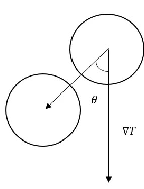
collision when the bubbles begin to “dance” with one another. Sanada et al. [ 2 ] in their 2005 study observed that an increasing Weber (We) number lead to a bubble bouncing off a free surface which in effect lengthens the coalescence time. A later study in 2009 by Sanada et al. [ 18 ] showed that the critical Reynolds (Re) number over which bubbles bounced decreased with an increase in Mo. They also showed that irrespective of the Mo value, a critical We value for bouncing was approximately equal to 2.0. It is important to note that for both Re and We in the 2009 study that a vertical rise velocity was used to calculate the non-dimensional numbers. Unlike the previous experiments, Kang et al. [ 19 ] performed an experiment that did not use non-dimensional numbers. They measured the effects of nonuniform temperature distribution on bubble coalescence. They found that because of thermocapillary forces from the nonuniform temperature, it caused one of the bubbles to glide over the surface of the other bubble which resulted in a coalescence probability distribution based on coalescence angle. It was observed that the highest probability of coalescence occurred between 20° − 40° angle. The angle between the temperature gradient and line connecting the bubble centers (See Figure 3).

(17)

transport equation to find source terms which can be calculated in a CFD code. This results in a more robust CFD code to predict evolution of bubble sizes. Mattson and Mahesh [ 24 ] took the expression of coalescence time scale from the previous model by Kamp et al. [ 22 ] and used it to develop a probability of coalescence. They then validated it using the result form Colin et al. [ 20 ] and find excellent agreement between the bubble size distributions. For a more comprehensive review of CFD studies on bubble coalescence, one is referred to Olmos et al. [ 25 ], Sommerfeld et al. [ 26 ], and van den Hengel et al. [ 27 ]. However, since CFD codes use approximations, they are unable to account for all of the fluid and bubble behavior and require DNS studies [ 24 ], [ 28 ].

Figure 3: The picture shows how the coalescence angle is defined.

(18)

referred to Crowe et. al. [ 30 ]. For DNS simulations, many different methods have been proposed to track the bubble interfaces including the Front-Tracking (FT) method, the Volume-of-Fluid (VOF) method, the Lattice Boltzmann (LBM) method, and the Level-Set (LS) method. The majority of the mention methods inherently incorporate coalescence of bubbles without any issue. The FT method however uses two separate grids for the two different phases and is unable to represent coalescence without a subgrid model. The VOF method can simulate coalescence but it is difficult to calculate the curvature from the front using volume fractions. Van Sint Annaland et al. [ 31 ] and Sussman et al. [ 32 ] provide a more comprehensive review of each of the above mentioned interface tracking methods. For more specific review of the FT, VOF, and LBM, one is referred to the following: Unverdi and Tryggvason [ 33 ], van Sint Annaland et al. [ 31 ], and Dabiri et al. [ 29 ] for FT, van Sint Annaland et al. [ 34 ] and Passandideh-Fard et al. [ 35 ] for VOF, and Takada et al. [ 36 ] and Inamuro et al. [ 37 ] for LBM.

(19)

in the simulation just as seen in the experiment (See Figure 4). It was also determined that the We number causing bouncing is constant and that the coalescence time increases with increasing We number. Yang et al. [ 40 ] continued development with the LS method by combining it with the VOF method to make a hybrid called the adaptive coupled level-set/volume-of-fluid (ACLSVOF) method. They found that ACLSVOF took advantage of the strengths of both the LS and VOF methods by making the surface tension calculations easier and more accurate while also keeping the mass conserved accurately. Yu and Fan [ 41 ] also studied the accuracy of the LS method. They performed simulations for a bubble rising in an infinite liquid by means of the buoyancy force in a three dimensional environment. They investigated the bubble shapes based on the Re and found good agreement between their simulations and experimental results. They also studied the shape of bubbles during coalescence with the LS method and noted a deviation in the shape of the second bubble compared with a single bubble case. They mentioned that no successful method has been developed to portray bouncing and coalescence based on the dynamic conditions of when they collide and that whether the bubbles will coalesce or bounce must be decided before the simulation is run.

2.2 Level-Set Method Overview

(20)

look into the LS method, the following section has been taken from a paper written by Bolotnov et al. [ 42 ] to provide the necessary background.

Figure 4: Plot reproduced from data reported by Sanada et. al [ 2 ]. The above plot is a comparison of experimental results and calculations. It shows that their simulation was able to closely model what was observed by Kirkpatrick and Lockett [ 16 ].

The level set method of Sussman [ 43 ], [ 44 ], [ 32 ] and Sethian [ 45 ] involves modeling the interface as the zero-level set of a smooth function, φ, where φ is often called the first scalar and it represents the signed distance from the interface. Hence, the interface is defined by φ = 0. The scalar, φ, is convected within a moving fluid according to,

0

D

u Dt t

 _  _{  }_

 ( 1 )

where u is the flow velocity vector. Phase-1, the liquid phase, is indicated by a positive level set, φ > 0, and phase-2, the gas, by a negative level set, φ < 0. Since evaluating the jump in

-4 -3.5 -3 -2.5 -2 -1.5 -1 -0.5 0

-0.03 -0.01 0.01 0.03 0.05

y/d

Time (sec)

(21)

physical properties using a step change across the interface leads to poor computational results, the properties near an interface were defined using a smoothed Heaviside kernel function (See Figure 5), Hε, given by [ 32 ]:

, 0

1 1 _,

( ) 1 sin

2 , 1 H     _{ }           _ _    _ _ _   _ __       

( 2 )

where ε is the interface half-thickness.

Figure 5: A plot of the smoothed Heaviside function that represents the transition of gas to liquid fluid properties

The fluid properties are then defined as:

1 2

( )

H

_

( )

(1

H

_

( ))

  



 







( 3 )

1 2

( )

H

_

( )

(1

H

_

( ))

  



 







( 4 )

-0.2 0 0.2 0.4 0.6 0.8 1 1.2

-0.3 -0.2 -0.1 0 0.1 0.2 0.3

φ

( )

(22)

The surface tension transition between the fluids is defined by:

𝛾𝜅𝛿(𝑛)𝒏 = 𝛾𝜅(𝜑)𝑑𝐻𝜀(𝜑)

𝑑𝜑 ∇(𝜑) ( 5 )

Although the solution may be reasonably good in the immediate vicinity of the interface, the distance field may not be correct throughout the domain since the varying fluid velocities throughout the flow field distort the level set contours. Thus, the level set was corrected with a re-distancing operation by solving the following PDE [ 44 ]:

( ) 1

d

S  d



 _ _{   }

 

 ( 6 )

where d is a scalar that represents the corrected distance field and τ is the pseudo time over which the PDE is solved to steady-state. This may be alternately expressed as the following transport equation:

( )

d

w d S 



 _{  }

 ( 7 )

The so-called second scalar, d, is originally assigned the level set field, φ, and is convected with a pseudo velocity, w, where,

( ) d w S

d

  

 ( 8 )

and S(φ) is defined as:

1 ,

1 _,

( ) sin

, 1 d d d d d S     _{ }           _ _    _ _  _ __        

(23)

where 𝜀𝑑 is the distance field interface half-thickness which, in general, may be different from

ε used in Eq. ( 2 ). Note that the zeroth level set, or interface, φ = 0, does not move since its convecting velocity, w, is zero. Solving the second scalar to steady-state restores the distance field to  d 1but does not alter the location of the interface. The first scalar, φ, is then updated using the steady solution of the second scalar, d.

Sussman et al. [ 32 ] and Sussman and Fatemi [ 44 ] proposed an additional constraint to be applied during the re-distancing step to help ensure the interface (φ = 0) does not move. It has been found in the present work that imposing this constraint also improves the convergence of the re-distancing step. The essence of the constraint is to preserve the original volume (i.e., mass) of each phase during the re-distance step.

The re-distancing step of the LS method is of vital importance to the coalescence control algorithm. It is necessary that the LS distance field contours return to the proper step after the advection of the velocity field since the curvature of these contours is used in identifying coalescence events.

CHAPTER 3 ALGORITHM DEVELOPMENT

(24)

the calculations were only performed on half of the domain. If the largest bubble diameter were used and the same resolution was applied to a small 3D domain of 20mm x 10mm x 10mm used in PHASTA simulations, the resolution would be 400 x 200 x 200 (16M elements) which is much finer than the finest resolution used in PHASTA of 160 x 80 x 80 (1M elements) for a 5 mm diameter bubble. This much finer mesh for the small 3D domain is feasible but this domain contains only two bubbles.

The goal is to prevent coalescence or model the coalescence dynamics for hundreds of bubbles. If the two bubble domain is taken as a standard, it would need to be 50 times larger to allow for 100 bubbles resulting in a 1000mm x 10mm x 10mm domain. Using the resolution from Sanada et al., this would create a resolution of 20000 x 200 x 200 (800M elements) for one hundred 5 mm diameter bubbles. The computational cost would be much too high for a simulation of this size. This means another method is required to provide the physics of film drainage in the simulation of bubble coalescence.

3.1 Repulsive Force

(25)

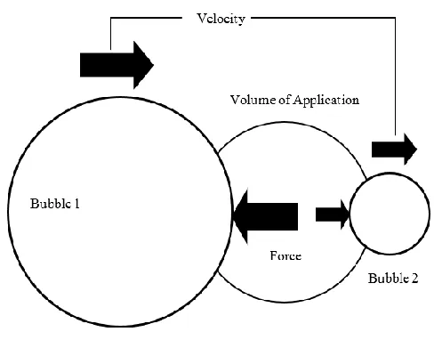
To apply this force, it was decided to locally increase the surface tension within a designated area of each bubble. The increase in surface tension was chosen because it was the most computationally affordable method to prevent coalescence compared with the other options (e.g. artificially increasing viscosity between the bubbles which requires much larger mesh resolution). Since the surface tension is not adjusted uniformly, this results in net force acting on each bubble in the direction opposite to the coalescence path (See Figure 6, Figure 7, and Figure 8).

(26)

Figure 7: An initial time step with the coalescence control application volume shown as the white circle and the black circles as the bubble interfaces

Figure 8: An later time step after surface tension changed with the coalescence control application volume shown as the white circle and the black circles as the bubble interfaces

(27)

the magnitude of the force based on the distance between the bubbles. This scales the force acting on the bubbles based on the surface area that is subtended by the sphere. This seems to leave the least amount of impact on the accuracy of the simulation since the properties values are only changed in a local area around the event. Also, the change only lasts as long as the bubbles are close to one another.

(28)

3.2 Location Identification

One of the importance aspects of this algorithm is to identify the location of a coalescence event. It is necessary to know the event location to be able to prevent or simulate the coalescence properly. One simple method to find the location is to use the distance field contours generated by the LS method in the PHASTA code. By using the distance field contours, it makes it possible to identify not just one coalescence event but multiple events simultaneously. However, it is beneficial to initially consider one coalescence event because it explains some of the basic principles necessary to detect multiple coalescence events at one time.

3.2.1 Single Event

(29)

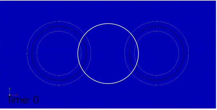
Figure 9: The distance field of the bubbles shown as the white contour lines with the black circles representing the bubble interface

(30)

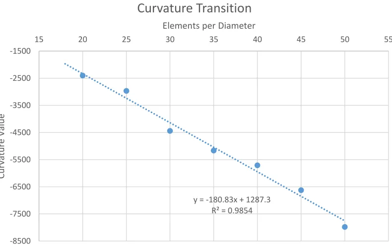
The current algorithm uses jumps in curvature between the first and sixth distance field contour. The limiting curvature values used to determine the coordinates has been determined empirically. A set of simple two bubble simulations, similar to the setup above, were used (See Figure 10). Each simulation in the set used a different resolution with 5 mm bubbles. The curvature values between the first and sixth distance field contour were recorded. A curvature value close to each jump in curvature was then taken and plotted against the number of elements across the bubble diameter (See Figure 11). A linear fit was then used to obtain an equation to calculate the limiting curvature value. As a buffer, this limiting curvature value was also multiplied by 1.45 to make sure intersecting contour coordinates were the only points tagged.

y = -180.83x + 1287.3 R² = 0.9854

-8500 -7500 -6500 -5500 -4500 -3500 -2500 -1500

15 20 25 30 35 40 45 50 55

Curv

at

u

re

Valu

e

(31)

Since it is possible to run PHASTA in parallel, multiple processors will contain an array with the recorded coordinates. These coordinate arrays from each processor are consolidated into three separate arrays distinguished by axis direction. The tag array from each processor is also consolidated into a single array. Each element of the coordinate arrays are summed and averaged by using the summation of the elements in the tag array. The average coordinates are the center coordinates for the two concentric circles generated by the intersecting contours. Since it is assumed there is only one coalescence event, the center coordinates identify the location of the event and can be used as the midpoint between the two approaching bubbles. A summary of the process can be seen in the following block diagram (See Figure 12).

Figure 12: Summary of process to identify a coalescence event and calculate the average coordinates for the event.

Step 1:

Check curvature to identify coordinates and tag array

location

Step 2:

Consolidate each processor coordinate array into the proper

axis array or tag array

Step 3:

Sum the elements of each axis array and the elements of the

tag array to get 3 total coordinate values and 1 tag value

Step 4:

Calculate the average coordinates for each axis by dividing

(32)

3.2.2 Multiple Events

The previously described method works in the case of just one coalescence event but fails to identify multiple events occurring simultaneously. To identify more than one location at a time, an extension of the previously described method is required. A summary of the following process can be seen in the block diagram of Figure 13. To determine if there are multiple events occurring simultaneously, the average vector distance from the average coordinates to the coalescence events coordinates is calculated. If this distance is larger than the contour diameter distance, then it signifies there are multiple coalescence events in the domain.

If it has been determined that multiple events are occurring simultaneously, it is necessary to sort and tag the coalescence events specific to each event. For multiple coalescence events, the average coordinates found from all of the intersecting contour coordinates is located at a point between all of the different coalescence events. This location is not necessarily centered between all the events because the averaging process used in steps 3 and 4 do not use any weights based on the number of coordinates recorded from each event. By knowing this location and the coordinates from each of the coalescence events, it possible to generate vectors that start at this averaged location and extend to each coalescence event coordinate.

(33)

than the diameter of the farthest chosen level set contour for event identification. The distance between an event coordinate and the coordinate of the maximum length vector can be calculated by using vector addition and then calculating the magnitude of the resulting vector. If the resulting vector is less than or equal to the diameter of the farthest chosen contour for the event identification, then there is a high probability that the coordinate belongs to the specific coalescence event.

Figure 13: Summary of process to find the average coordinates for each specific coalescence event during multiple coalescence events.

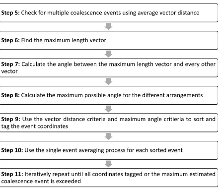
Step 5:Check for multiple coalescence events using average vector distance

Step 6:Find the maximum length vector

Step 7:Calculate the angle between the maximum length vector and every other vector

Step 8:Calculate the maximum possible angle for the different arrangements

Step 9: Use the vector distance criteria and maximum angle critieria to sort and tag the event coordinates

Step 10:Use the single event averaging process for each sorted event

(34)

Since it is not possible to assuredly determine that a coordinate belongs to a specific coalescence event using the vector comparison, the angle between each vector and the maximum length vector for a specific coalescence event is used as the second criteria. By using the farthest chosen contour diameter from which coordinates are tagged, it is possible to calculate the maximum angle that would exist between the longest vector for a specific coalescence event and another vector resulting in a triangle with the contour diameter and maximum length vector. A geometric representation of this scenario can be seen in Figure 14.

Figure 14: Triangle formed by three vectors during multi-event coalescence identification.

(35)

used to determine the maximum angle at which the vectors can be positioned for each arrangement (See Eqs. ( 10 ), ( 17 )).

Arrangement 1: Sides c and a are known

The first arrangement occurs when side c represents the maximum length vector and side a represents the contour diameter. The form of the law of cosines used for this arrangement is the following:

𝑎2 _{= 𝑏}2_{+ 𝑐}2_{− 2𝑏𝑐 ∗ cos(𝛼)} _{( 10 )}

Since the largest possible value of 𝛼 is needed as a criteria, the length of 𝑏 must be determined when 𝛼 is maximized. To do this, Equation ( 10 ) is solved for 𝛼 and the first derivative of 𝛼

is taken with respect to 𝑏 (See Eqs. ( 11 ) and ( 12 )).

α = cos−1(𝑏

2_{+ 𝑐}2_{− 𝑎}2

2𝑏𝑐 ) ( 11 )

𝑑𝛼 𝑑𝑏 = −

1

√1 − (𝑏2− 𝑐2+ 𝑎2 2𝑏2_𝑐 )

2

(𝑏

2 _{− 𝑐}2_{+ 𝑎}2

2𝑏2_𝑐 )

( 12 )

In order to maximize 𝛼, 𝑑𝛼

𝑑𝑏 is set equal to zero. From Equation ( 12 ), there are two possibilities

that would make 𝑑𝛼

𝑑𝑏 equal to zero:

− 1

√1 − (𝑏2− 𝑐2+ 𝑎2 2𝑏2_𝑐 )

2

= 0

(36)

(𝑏

2_{− 𝑐}2_{+ 𝑎}2

2𝑏2_𝑐 ) = 0 ( 14 )

For Equation 4 to be true, 𝑏 must be equal to infinity. This does not make sense for a finite triangle which means Equation 5 must be used. This equation is solved for 𝑏 to calculate the length of 𝑏 to maximize 𝛼:

𝑏 = √𝑐2_{− 𝑎}2 _{( 15 )}

Equation 6 is just a modified form of the Pythagorean Theorem which means that 𝛼 is maximized when vectors 𝑎, 𝑏, and 𝑐 form a right triangle. Since the vectors form a right triangle, 𝛼 can be calculated using a basic trigonometric function:

𝛼 = cos−1(𝑏

𝑐) ( 16 )

Arrangement 2: Sides c and b are known

Within this arrangement, there are two possible setups. The first occurs when the maximum length vector is still acting as 𝑐 but the farthest chosen contour diameter is represented by side

𝑏. For this arrangement, the angle 𝛽 is maximized instead of the angle 𝛼. For this arrangement, the following form of the law of cosines is used:

𝑏2 = 𝑎2+ 𝑐2− 2𝑎𝑐 ∗ cos(𝛽) ( 17 ) The same process is followed as in Arrangement 1 but 𝑑𝛽

𝑑𝑎 is found in order to maximize 𝛽.

When calculated, you get a function of the same form as Equation 3. Here 𝑑𝛽

𝑑𝑎 is set equal to

(37)

𝑎 = √𝑐2 _{− 𝑏}2 ( 18 ) Again, this equation is an alternate form of the Pythagorean Theorem. This means that simple trigonometric functions can be used to solve for the maximum of angle 𝛽:

𝛽 = sin−1₍𝑏

𝑐) ( 19 )

The second setup of this arrangement is where the contour diameter acts as side 𝑐 and the maximum length vector acts as side 𝑏. In this instance, the average coordinate may be located within the sixth contour of one of the bubbles. This represents a situation where this coalescence event generates many more event coordinates than other events. In the extreme, it is possible that the average coordinates could be at the center of the coalescence event. However, it is assumed that the number of event coordinates does not significantly outweigh other events so it is assumed that the maximum angle of 𝛾 occurs when the length of a line drawn from point 𝐶 in Figure 14 and perpendicular to side 𝑐 is equal to the bubble radius plus one contour distance (See Figure 15).

With this assumption, it is not possible to assume that the triangle formed is a right triangle. The line drawn between point 𝐶 and perpendicular to side 𝑐 can be used since this forms two right triangles. This means that the angle 𝛾 and the side 𝑐 can be broken into two pieces:

𝛾 = 𝜃 + 𝜙 ( 20 )

𝑐 = 𝑙 + 𝑚 ( 21 )

This means that 𝜃 and 𝜙 can be found by the following equations:

𝜃 = cos−1(𝑑

(38)

𝑙 = 𝑏 ∗ sin (𝜃) ( 23 )

𝑚 = 𝑐 − 𝑙 ( 24 )

𝜙 = tan−1(𝑚

𝑑) ( 25 )

The angle 𝛾 can then be used as the maximum angle between the maximum length vector and any other vector.

Figure 15: Schematic of triangle to calculate the angle gamma when the sides b and c are known.

Now that the maximum angles can be calculated, it is necessary to calculate the angles between the maximum length vector and every other vector in order to compare the angles as the second criteria. To calculate the angles, the definition of the dot product between two vectors is used:

𝜓𝑖 = cos−1(

𝑐 ∙ 𝑣𝑖

(39)

where 𝑐 is the largest length vector, 𝑣𝑖 is any other vector, and 𝜓𝑖 is the angle between the

largest length vector and any other vector.

Once each of the values for the criteria have been calculated, they can be used to sort and tag the event coordinates specific to each coalescence event. This process will occur iteratively until all event coordinates have been tagged or the maximum number of estimated coalescence events has been exceeded. Once all the iterations have completed, the same averaging process used for a single coalescence event is used for each tag separately. This results in an array of center coordinates for each set of concentric circles generated by the different coalescence events and therefore identifies each event separately.

3.3 Drainage Time

Once the coalescence event has been identified and the force is implemented, it is necessary to track the amount of time the force has been active. The tracked time can then be compared to a coalescence time model [ 7 ] that estimates the total coalescence time. Once the tracked time has exceeded the estimated total coalescence time, the force is removed, signifying the liquid film has had sufficient time to drain, and the bubbles are allowed to coalesce.

The drainage time uses a model that is based on the equivalent bubble radii (𝑟_𝑖𝑗), the density of the liquid (𝜌_𝑙), the surface tension (𝜎), and the initial and final film thickness (ℎ_𝑜, ℎ_𝑓):

𝑡_𝑖𝑗 = √𝑟𝑖𝑗

3_𝜌 𝑙

16𝜎ln ( ℎ𝑜

ℎ𝑓

) ( 27 )

(40)

𝑟𝑖𝑗 =

1 2(

1 𝑟𝑏𝑖

+ 1 𝑟𝑏𝑗

)

−1

( 28 )

where the indices 𝑖, 𝑗 represent different bubbles. The initial film thickness is estimated as 1 ∗ 10−4_𝑚_{by Kirkpatrick and Lockett [ 16 ] and the final film thickness is usually taken to be}

1 ∗ 10−8 𝑚 [ 11 ].

To track the coalescence events, it is necessary to develop several logic loops in order to: identify new coalescence events, keep track of the continuing events that have and have not exceeded the model time limit, and determining when events have ended whether through coalescence or the bubbles moving away from (bouncing off) one another. Since each event is not assigned the same event number after each iteration, the distance between the average coordinates from the previous iteration and the current iteration are used to identify which events are the same. The distance between the average coordinates will always be quite small. The default values for the average coordinates are used to help identify when any new and ending events occur.

CHAPTER 4 SIMULATIONS

(41)

4.1 Two Bubble Coalescence Prevention

The first simulation consists of how the algorithm handles when there is only one coalescence event occurring in the domain. The time tracking portion of the algorithm was not tested in this simulation. The domain size was 40 mm x 20 mm x 20 mm with the x-y planes acting as walls. There were three bubbles placed in the domain: (i,ii) two bubbles with a 5 mm diameter and (iii) a third with a 6 mm diameter. The bubbles were placed at varied distances in the x-direction along the center line between two parallel plates. Gravity was used to provide a buoyance force on the bubbles to cause them to flow while a pressure gradient was applied to the liquid to keep it stationary within the domain. A finite element mesh containing 2M hexahedral elements. This means that the 5 mm diameter bubbles were resolved with at least 25 elements across its diameter. For more information on the domain and simulation parameters, see Figure 16 and Table 1.

The simulation was used for two tests. The first test was performed without using the coalescence control algorithm. The second test was performed with the coalescence control active. To analyze how the algorithm handles a single event, only the interaction between the two 5 mm diameter bubbles is considered.

(42)

Figure 16: Initial setup to test the algorithm for a single coalescence event identification and prevention.

Table 1: Overview of simulation parameters for the single coalescence prevention simulation.

Parameter

Liquid water

Gas air

Pressure, Pa 0

Temperature, °C N/A (0)

Liquid Density, kg/m3 997.17

Gas Density, kg/m3 _1.161

Liquid viscosity, kg/m-s 2.67E-03

Gas viscosity, kg/m-s 1.86E-02

Body Force, m/s² 0.5

Body Force Pressure Gradient, Pa/m 498.585

(43)

coalescence control. Even though the coalescence control increases the computational cost, this increase is cost is manageable and willing trade off to the resolution required for coalescence viscosity effects to be observed.

(a) (b) (c)

Figure 17: Visualization of the simulations for the single coalescence events at iterations: (a) 20, (b) 400, and (c) 870. Top: The simulation performed without the coalescence control algorithm. In iteration 870, the 5 mm bubbles have begun to coalesce. Bottom: The simulation performed with the coalescence control algorithm. In iteration 870, the coalescence event has been prevented.

4.2 Multi-Bubble Coalescence Prevention

(44)

across the diameter of the bubbles. For more information on the simulation parameters and the domain, see Figure 18 and Table 2.

Figure 18: Overview of the simulation domain dimensions and axis orientation. The shaded planes represent walls.

The described simulation was tested twice: one without using the coalescence control algorithm and one with the coalescence control algorithm active. The starting point for these tests started at iteration 7800 (See Figure 19). To determine if bubble coalescence events have occurred, later iterations were chosen and the number of bubbles was counted. The iterations that were chosen were matched based on time within the simulation. The times

2δ = 2.0

x z y

g

(45)

Table 2: Overview of simulation parameters for the multi-bubble coalescence prevention simulation.

Parameter

Pressure, bar 10

Liquid water

Gas air

Temperature, °C 27

Liquid Density, kg/m3 996.5 Gas Density, kg/m3 11.636 Liquid viscosity, kg/m-s 8.514∙10-4

Gas viscosity, kg/m-s 1.858∙10-5

Figure 19: Initial setup at iteration 7800 of the bubbly flow in turbulent conditions. There are 32 bubbles randomly placed throughout the domain.

(46)

(47)

(a) (b) (c)

(48)

4.3 Coalescence Time Tracking

The third test simulation was designed to test the coalescence control algorithm’s time tracking model. This simulation design consists of a single bubble below a free surface of gas placed at the top of the domain. The domain size was 20 mm x 35 mm x 20 mm. The bubble diameter was 5 mm and the center point of the bubble was placed 20 mm below the free surface (See Figure 21). Gravity was used to provide a buoyance force to force the bubble to approach the free surface. A wall was placed on the top and bottom of the domain normal to the gravity and buoyance force. The mesh was made of 0.9M hexahedral elements resulting in approximately 20 elements across the diameter of the bubble. For more information on simulation parameters, see Table 3.

Table 3: Overview of simulation parameters for the time tracking tests.

Parameter

Liquid water

Gas air

Pressure, Pa 0

Gas Density, kg/m3 _1.161

Body Force, m/s² 1

(49)

time tracking portion of the coalescence control was active. The first test was performed without using the time tracking portion of the code. It can be seen in iteration 800 that the force is implemented. Later, in iteration 1150, the simulation shows that the coalescence event has

Figure 21: Initial setup for the bubble rising towards a free surface. The simulation was used to test the time tracking portion of the algorithm.

(50)

(a) _(b) (c)

(51)

A new capability was used in these simulations so the computational cost changed from the previous simulations. Without the time tracking algorithm active, the simulation finished 1500 iterations in 2.33 hours. When the tracking algorithm was active, the simulation finished 1500 iterations in 2.36 hours. This signifies only a 1% increase in the running cost of adding the time tracking portion of the algorithm. This running cost increase is insignificant to the cost of running the rest of the coalescence control algorithm and is therefore an easy tradeoff.

CHAPTER 5 VERIFICATION AND VALIDATION

5.1 Mesh Study

(52)

Figure 23: Initial setup of the simulation used in the mesh study. The domain contains two 5 mm bubble.

Table 4: Overview of simulation parameters for both mesh types.

Parameter

Liquid water

Gas air

Pressure, Pa 0

Gas Density, kg/m3 1.161

Body Force, m/s² 0.5

(53)

complex and less efficient grid. The coalescence control algorithm will be used in both meshes and therefore a mesh study must be performed using both meshes.

5.1.1 Discrete Mesh

For this test, the interface half-thickness was kept at 4.5 ∗ 10−4 which is equal to 1.8 times a 20 point per diameter resolution. The bubbles in the diameter were setup such that the midpoint between them was set at (1.0E-2, 7.5E-3, 7.5E-3). Each simulation was run for five iterations and the coalescence event coordinates reported were taken from the third iteration.

(a)

(b)

(54)

The third iteration was chosen to allow the algorithm to perform a couple of iterations while not waiting too long such that the bubbles moved sufficiently to drastically move the coalescence event location. These coalescence event coordinates can be seen in Table 5. Each set of coordinates was compared to the exact midpoint value and the normalized based on the distance between the center points of the bubble (See Table 6).

Table 5: Contains the average coordinates for different discrete domain resolutions. It also contains the exact geometric coordinates and distance between bubble centers.

Reported Center Points for Coalescence Events in Discrete Simulation

3rd Iteration Coordinates

Exact Bubble Center Distance 20 Pts. 25 Pts 30 Pts. 35 Pts. 40 Pts.

X Coord 1.01E-02 1.01E-02 1.00E-02 1.00E-02 1.00E-02 1.00E-02 9.00E-03

Y Coord 7.49E-03 8.08E-03 8.32E-03 7.89E-03 8.21E-03 7.50E-03 9.00E-03

Z Coord 7.49E-03 7.11E-03 6.85E-03 7.07E-03 7.38E-03 7.50E-03 9.00E-03

Table 6: Contains the error between the reported coordinates and the exact geometric coordinates normalized by the distance between bubble centers.

Percent Error Normalized by Distance between Bubble Centers

20 Pts. 25 Pts 30 Pts. 35 Pts. 40 Pts.

X Coord 1.006611539 0.67252167 0.409646053 0.510499203 0.451368364 Y Coord 0.081854474 6.452301016 9.107695555 4.34685935 7.86000409 Z Coord 0.086528576 4.298314523 7.271514561 4.79368714 1.344575277

(55)

distributed. This would cause a skew in the average y and z coordinates without affecting the x coordinate.

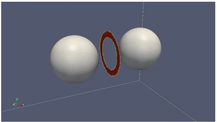
To determine whether the errors affect the outcome in later iterations, the 20 elements and 40 elements across the 5 mm bubble diameter simulations were run longer. These simulations were performed for 500 iterations each. The 250th iteration was chosen for the 20 element resolution since the simulation matched the 500th iteration of the 40 element resolution. As expected for the 20 elements per diameter resolution, the coalescence event was prevented (See Figure 25 (a)). It can also be seen in Figure 25 (b) that the coalescence event was prevented in the 40 element resolution as well. This shows that the errors in the higher resolution are insufficient to cause the algorithm to work improperly.

(a) _(b)

(56)

5.1.2 Parasolid Mesh

For this test, the interface half-thickness was kept at 3.0 × 10−4_{which is equal to 1.8 times}

a 30 point per diameter resolution. The bubbles in the diameter were setup such that the midpoint between them was set at (1.0E-2, 0, 0). Again, each simulation was run for five iterations and the coalescence event coordinates reported were taken from the third iteration. These coalescence event coordinates can be seen in Table 7. Each set of coordinates was compared to the exact midpoint value and normalized based on the bubble center distance (See Table 8).

Table 7: Contains the average coordinates for different parasolid domain resolutions. It also contains the exact geometric coordinates and distance between bubble centers.

Reported Center Points for Coalescence Events (30 Pts. Eps.)

3rd Iteration Coordinates

Exact

Bubble Center Distance 20 Pts. 25 Pts 30 Pts. 35 Pts. 40 Pts.

X Coord 1.01E-02 1.00E-02 1.00E-02 1.01E-02 1.01E-02 1.00E-02 7.20E-03

Y Coord 5.87E-05 4.23E-05 4.50E-05 3.08E-04 6.15E-04 0.00E+00 7.20E-03

Z Coord 1.18E-05 -1.69E-08 -4.81E-05 7.92E-04 1.21E-03 0.00E+00 7.20E-03

Table 8: Contains the error between the reported coordinates and the exact geometric coordinates normalized by the distance between bubble centers.

Percent Error Normalized by Distance between Bubble Centers

20 Pts. 25 Pts 30 Pts. 35 Pts. 40 Pts.

(57)

Among all the cases, the highest error was seen to be about 16%. The largest error were only seen in the y and z coordinates. This result shows high accuracy with the expected results. The higher error in the y and z coordinates can be explained by the same reasoning in the discrete domain. The y and z average coordinates are generated from intersecting contours in the y-z plane. It is possible that the concentration of points found around the intersecting contours was not evenly distributed. This would cause a skew in the average y and z coordinates without affecting the x coordinate.

To determine whether the errors affect the outcome in later iterations, the same process was used as with the discrete mesh. The two simulations of 20 elements and 40 elements across the 5 mm bubble diameter were performed for 500 iterations each. Visualizations of each case was chosen based on matching time within the simulation (See Figure 26). For these two simulations, the interface half-thickness was not a proper match. However, for both simulations, the coalescence event was still prevented (See Figure 26). This shows that the errors due to a mismatched interface half-thickness are insufficient to make the algorithm work improperly.

5.2 Minimum Liquid Film Thickness during Coalescence Control

As mentioned earlier, the initial distance estimated by Kickpatrick and Lockett [ 16 ] was

(58)

towards a free surface simulation (See Section 4.3). The same domain and simulation parameters were used (See Figure 21 and Table 3).

(a) (b)

Figure 26: Visualization of the parasolid mesh study for the 20 element and 40 element resolution. (a) The 20 element resolution at iteration 280. (b) The 40 element resolution at iteration 500.

(59)

the original sixth distance. In order to be successful, the algorithm using closer contours still needed to prevent the coalescence event. The time application portion of the algorithm was not used for these tests since it was necessary to prevent the coalescence event for the test. The simulation setup and parameters were the same as those used in the coalescence time tracking section (See Section 4.3). For distance field contours closer than the fifth contour, the initial thickness for coalescence then becomes twice the distance to the specific contour. The distances for the three different tests can be seen in Table 9. When the original algorithm is used, it can be seen that the force is implemented in iteration 880 and the coalescence event was prevented by iteration 940 (See Figure 27 (a)). Changing the algorithm to activate at the fourth distance field contour was performed next. It can be seen in iteration 880 that the force is implemented. After the force had been implemented, it can be seen in iteration 940 that the coalescence event is prevented (See Figure 27 (b)). This means that the initial coalescence thickness could be reduced to 3.6 mm.

Table 9: Initial liquid film thickness based on which distance field contour is used to activate the coalescence control algorithm.

Initial Liquid Film Distance for Coalescence Events

Identification Contour Initial Thickness (mm) 5th Contour Application Diameter

3rd 2.7 4.5

4th 3.6 4.5

6th 4.5 4.5

(60)

iteration 940, the timing of the force application and force strength was insufficient in preventing coalescence between the bubble and free surface (See Figure 27 (c)). This shows that the third distance field contour is insufficient in preventing coalescence events. Even though it was unable to prevent the coalescence in this simulation, it may still be possible to make this algorithm perform successfully. To do this, the magnitude of the force must be increased which results in adjusting the surface tension within the application volume. This means the distance could be reduced even further. This shows that even though the original algorithm cannot accurately represent the initial coalescence thickness, it is possible to reduce the distance by adjusting some of the parameters used in the algorithm.

5.3 Initial and Final Bubble Diameter Distribution

(61)

(a) (b) (c)

(62)

5.4 Bubble Approach Velocity Effect on Coalescence

The second validation test to be performed for the algorithm uses the single bubble rising towards a free surface. This simulation design was based off the same setup as the simulation in coalescence time tracking testing (See Section 4.3 and Figure 21). However, the simulation will be modified to match an experiment performed by Kirkpatrick and Lockett [ 16 ]. A 5 mm diameter bubble will be placed in a liquid domain below a free surface of gas at the top of the domain. Two different distances below the free surface will be used: 45 cm and 67 cm. Gravity will be used to provide a buoyance force to force the bubble to approach the free surface. A wall will be placed on the top and bottom of the domain normal to the gravity and buoyance force. The mesh is made of 8.5M or 12.6M hexahedral elements resulting in approximately 18 elements across the diameter of the bubble. The Morton number (Mo) will be used to relate the adjusted simulation properties to the experimental properties (See Table 10).

Table 10: Overview of experiment and simulation parameters for the bubble approach velocity effect on coalescence simulation.

Parameter Experimental Simulation

Liquid water water

Gas air air

Pressure, Pa 0 0

Temperature, °C N/A (0) N/A (0)

Liquid Density, kg/m3 997.17 997.17

Gas Density, kg/m3 1.161 1.161

Liquid viscosity, kg/m-s 2.67E-03 3.57E-03

Gas viscosity, kg/m-s 1.86E-02 1.86E-02

Body Force, m/s² 9.81 1

(63)

These tests will be performed with the time tracking portion of the code active. The results will be compared to the experimental results of Kirkpatrick and Lockett [ 16 ]. They observed that for bubble to free surface distances less than 61 cm the coalescence process was almost immediate. However, for distances larger than 61 cm, the coalescence process was much longer. By the time the bubble first makes contact with the free surface, it had gained sufficient speed to bounce off the free surface before coalescing. The coalescence time model taken from Prince and Blanch [ 7 ] did not take bubble approach velocity into account. However, testing this capability of the algorithm will help determine which simulations can be expected to provide proper physical results.

CHAPTER 6 CONCLUSION

6.1 Discussion

An algorithm was developed for the LS method that represents the effect of liquid film drainage during a coalescence event. Instead of using a high resolution grid to simulate the viscous drainage of the film, it prevents or slows the coalescence process by applying a force to both bubbles. The force is generated by locally changing the surface tension on a portion of each interface. This method was tested for single and multiple coalescence events in both laminar and turbulent flow regimes. In both cases, the algorithm successfully identified coalescence events and prevented the bubbles from coalescing.

(64)

rising towards a free surface. The time tracking portion of the code successfully removed the locally modified surface tension allowing the bubble and free surface to coalesce.

We have observed some non-critical issues with the algorithm. One of these issues pertains to the deformation of the bubble interface. When the surface tension is changed, that portion of the bubble begins to flatten. In some situations, this is a physical process (e.g. representing the effect of the liquid film and the other interface on the bubble). However, the algorithm applies the changed surface tension before the liquid film is sufficiently thin to cause the flattening of the surface. Another issue is related to the initial film thickness that develops between the bubbles. With a moderate resolution, the initial thickness generated by the coalescence control algorithm is equal to 4.5 mm. This is much larger than the estimated thickness of 0.1 mm by Kirkpatrick and Lockett [ 16 ]. However, it has been demonstrated that the initial thickness can be reduced by adjusting parameters within the coalescence control algorithm. For multiple bubble simulations it is way more important to maintain the correct coalescence probability then to correctly resolve the thinnest film when the bubbles bounce off each other. Even with these minor issues, the presented coalescence control algorithm is the only feasible way to simulate multiple bubble behavior using LS approach at large scale.

6.2 Future Work

(65)

travel through a periodic boundary, some of the area near the boundary retains the changed surface tension. The changed surface tension would then change the trajectory of some of the bubbles as they pass through the boundary. The problem is probably caused by the way the boundary values are updated after each iteration. More work would need to be done in finding out how the changed surface tension and boundary conditions interact.

Another possible change in the algorithm that can make it more robust is developing an analytical model to determine the expected curvature for intersecting contours. The current method was developed empirically by analyzing the curvature values for a simple two bubble simulation. Multiple cases were performed where each the resolution was adjusted between each case. There is a significant jump in magnitude for curvature values where the distance field contours intersect. A curvature value close to the curvature jumps was chosen for each resolution. These values were then plotted against the resolution and an equation was generated using a linear fit (See Figure 11). The algorithm then uses this equation and multiplies the resulting values by 1.45 for a buffer to generate the limiting curvature values. Developing the analytical analysis will make the identification of the coalescence event locations more accurate.

(66)

third option would be to change the surface tension profile across the application volume. Currently, the surface tension is adjusted uniformly throughout the application volume. Instead of using a constant profile, a quadratic or exponential profile could be used. This would then reduce effect on the coalescence process until both bubbles have moved farther into the application volume. This would then allow the force to be implemented within a volume between the bubbles that is much thinner than the spherical volume. Finally, time dependent coalescence control force can be introduced which will monitor the bubble velocities and change its value based on the bubble dynamics. Adjusting the algorithm in such a way would allow the method to simulate the coalescence process closer to what is observed experimentally.

Another option to make the algorithm simulate coalescence events with increased accuracy would be to update the coalescence time model used. The model developed by Prince and Blanch [ 7 ] was developed without considering the approach velocity of the bubbles. It was also not able to accurately predict coalescence rates when electrolyte solutions with salt concentrations past the transition concentration. The inability of the model to predict the rates was attributed to the effects of turbulence on surface mobility, the dynamics of bubble collisions, and the solute concentration at the gas-liquid interface of the coalescing bubbles. A better time model that includes these effects could be implemented to make the time tracking portion of the algorithm closer to experimentally observed values.

(67)

information on the bubble radius is built into the distance field. By investigating other parts of the PHASTA code, it would be possible to pull the radius from the distance field information instead of providing it manually. The estimated number of coalescence events is used to determine how many times to loop through the portion of the code that identifies multiple coalescence events. Manually providing this looping value is not the most computationally efficient. The algorithm could be smarter by developing a portion of the algorithm to adjust this looping value. It would simple to decrease the looping value if some of the average coordinate values are not changed from the default value for a specific number of time steps. It would require more work to add to the looping value if more coalescence events then being identified are occurring. However, these adjustments would make the algorithm more robust and easier to use.

For future development and study, the algorithm could be analyzed for simulations when the bubbles are no longer spherical. Since the algorithm uses the curvature of the distance field to identify coalescence events. However, bubbles are only spherical at very small flow velocities or very small diameters. This adjustment to the algorithm will be necessary if the study wants some bubbles to coalesce. These coalescence events will increase the bubble diameter which may make it large enough to start deforming. However, it is undesirable for the algorithm to identify a false coalescence event due to sharp curvature changes in the bubble shape.

(68)

(69)

REFERENCES

1. Bolotnov, I. A., Jansen, K. E., Drew, D. A., Oberai, A. A. & Lahey, Jr., R. T., Detached Direct Numerical Simulation of Turbulent Two-phase Bubbly Channel Flow. Int. J. Multiphase Flow 37, 647-659 (2011).

2. Sanada, T., Watanabe, M. & Fukano, T., Effects of viscosity on coalescence of a bubble upon impact with a free surface. Chemical Engineering Science 60, 5372-5384 (2005). 3. Chen, J.-D., Hahn, P. S. & Slattery, J. C., Coalescence time for a small drop or bubble

at a fluid-fluid interface. AIChE Journal 30 (4), 622-630 (1984).

4. Lee, J. C. & Hodgson, T. D., Film flow and coalescence - I basic relations, film shape and criteria for interface mobility. Chemical Engineering Science 23, 1375-1397 (1968).

5. Li, D., Coalescence between two small bubbles or drops. Journal of Colloid and Interface Science 163, 108-119 (1994).

6. Marrucci, G., A theory of coalescence. Chemical Engineering Science 24, 975-985 (1969).

7. Prince, M. J. & Blanch, H. W., Bubble coalescence and break-up in air-sparged bubble columns. AIChE Journal 36 (10), 1485-1499 (1990).

8. Marrucci, G. & Nicodemo, L., Coalescence of gas bubbles in aqueous solutions of inorganic electrolytes. Chemical Engineering Science 22, 1257-1265 (1967). 9. Lessard, R. R. & Zieminski, S. A., Bubble coalescence and gas transfer in aqueous

electrolytic solutions. Ind. Eng. Chem. Fundam. 10 (2), 260-269 (1971).

10. Cain, F. W. & Lee, J. C., A technique for studying the drainage and rupture of unstable liquid films formed between two captive bubbles: measurements on KCL solution. Journal of Colloid and Interface Science 106 (1), 70-85 (1985).

11. Kim, J. W. & Lee, W. K., Coalescence behavior of two bubbles in stagnant liquids. Journal of Chemical Engineering of Japan 20 (5), 448-453 (1987).