ABSTRACT
WHITE, JOSHUA D. African Easterly Wave Storm Track Dynamics. (Under the direction of Anantha Aiyyer).
This dissertation examines two factors that determine the structure and underlying dynamics of the African easterly wave (AEW) storm track. The first is the role of prominent features of North African orography and the second is the instability of the African easterly jet (AEJ).
Experiments are performed using a numerical weather prediction model for the AEW season with reduced orography in four key regions. R1 contains the Hoggar, Tibesti, and Darfur mountains, R2 contains the Cameroon highlands, R3 contains the Ethiopian high-lands, and R4 contains the Guinea highlands. Terrain reduction in R1, R2, and R3 leads to a reduction of the activity in the southern AEW storm track. On the other hand, only R1 reduction leads to a decrease in activity of the northern track AEW storm track. R4 reductions have minimal impact. The southern track reduction is connected to decreases in orographically induced convection. The attendant reduction in diabatic heating along the ITCZ impacts the generation of eddy available potential energy and baroclinic overturning that are needed for AEW development. The R1 reduction in the northern track is associated with decreased baroclinicity in vicinity of the northern track. Importantly, the results show that while elevated terrain features over Africa impact the overall storm track strength, they are not necessary for the generation of AEWs, contrary to the speculation in numerous past studies.
© Copyright 2019 by Joshua D. White
African Easterly Wave Storm Track Dynamics
by
Joshua D. White
A dissertation submitted to the Graduate Faculty of North Carolina State University
in partial fulfillment of the requirements for the Degree of
Doctor of Philosophy
Marine, Earth, and Atmospheric Science
Raleigh, North Carolina 2019
APPROVED BY:
Stuart Bishop Arlene Laing
Walter Robinson Carl Schreck
Anantha Aiyyer
ACKNOWLEDGEMENTS
First and foremost, I must thank my wife, Veronica Varela, for her unconditional support without which I could not have completed this work. She has been my source of motivation from the start, and no one thing she has done, small or large, has gone unnoticed. I would also like to thank my friends who have provided moral support and laughter along the way.
I would like to acknowledge my advisor, Dr. Anantha Aiyyer, for his guidance and support since the start of my degree. Thank you for taking a chance on a student from a non-traditional undergraduate degree and for sharing your enthusiasm with the field. I would also like to thank Dr. James Russell with whom I worked with and learned alongside as we pursued our degrees together. I would also like to thank the members of my committee for their thoughts and contributions throughout the completion of this dissertation.
TABLE OF CONTENTS
List of Tables. . . v
List of Figures. . . vi
Chapter 1 Introduction. . . 1
1.1 Definitions . . . 1
1.2 Motivations . . . 2
1.3 Background . . . 3
1.3.1 Early Understanding . . . 3
1.3.2 Recent Developments . . . 6
1.3.3 Local instability . . . 10
1.4 Research Objectives and Scientific Questions . . . 13
Chapter 2 The Impact of Orography on the Simulated African Easterly Wave Storm-track. . . 15
2.1 Background . . . 15
2.2 Methods . . . 18
2.3 Results . . . 20
2.3.1 Comparison to Reanalysis . . . 20
2.3.2 Stormtrack Sensitivity to Orography . . . 22
2.3.3 Energetics . . . 26
2.4 Discussion . . . 32
2.5 Conclusions . . . 35
2.6 Figures . . . 38
Chapter 3 Persistence of African Easterly Waves and the Instability of the African Easterly Jet . . . 61
3.1 Background . . . 61
3.2 Methods . . . 66
3.3 Results . . . 69
3.3.1 Climatological Basic State . . . 69
3.3.2 Composite Wave Responses . . . 72
3.3.3 Examples of Convective Instability . . . 78
3.3.4 Noise Forcing . . . 80
3.3.5 Seasonal Influence . . . 82
3.4 Conclusions . . . 83
3.5 Figures . . . 86
Chapter 4 Summary . . . 124
APPENDICES . . . 134
LIST OF TABLES
Table 2.1 EKE, EAPE, and energy budget terms averaged over -30 to 60◦E, -5 to 30
◦N, and from the surface to 300 hPa over JAS 2008-2017. The percentage
change from the control in the terrain reduction experiments are shown in parentheses, and∗indicates significance at 95% confidence level for the volume averaged quantities. The units for EKE and EAPE are J kg−1while the energy budget terms have units of J kg−1day−1. . . 32
Table 3.1 Categorization of the longevity of resulting wave packets in each of the fixed-heating simulations on the 775 15-day averages, separated every 5 days, from JJAS 1987-2017. . . 69 Table A.1 A summary of acronyms used in alphabetical order. . . 135 Table B.1 A summary of common meteorological variables and other symbols
LIST OF FIGURES
Figure 1.1 ERAi June-October, 1987-2017 averaged zonal winds (shaded, m s−1, in a,b) map at 650 hPa (a) and latitude-height cross section averaged over -15 to 15◦E (b) and meridional PV gradient (shaded, PVU 1000
km−1, in c,d) map at 650 hPa (c) and latitude-height cross section av-eraged over -15 to 15◦E (d). For comparison, zonal winds are overlaid
(contoured every 1 m s−1) in (c) and (d), with dashed lines indicating
easterly flow. Winds less than 6 m s−1are drawn with thicker markings to highlight the AEJ. . . 5 Figure 1.2 ERAi June-October, 1987-2017 averaged EKE (shaded, J kg−1) map at
650 hPa (a) and 925 hPa (b) and latitude-height cross section averaged over -15 to 15◦E (c). As in Figure 1.1, zonal winds (contoured every
1 m s−1) at 650 hPa are overlaid in (a,b) and from the -15 to 15◦E
average in (c). . . 6 Figure 1.3 Absolute (left) and convective (right) instability represented in the
x-t plane for an unstable easterly flow. Initially, a disturbance un-dergoes growth in an unstable region and disperses energy into a spreading wave packet as time increases. The spread of the wave packet is controlled by the total group velocityCg T of the disturbance
and is bounded byCg Tmin on the leading edge of the wave packet and
Cg Tmaxon the lagging edge of the wave packet. IfCg T =0 falls within
this cone, then there is both upstreamanddownstream development in the wave packet, and the flow is absolutely unstable. Otherwise, the flow is convectively unstable. Adapted from Diaz and Aiyyer (2015). 11 Figure 2.1 EKE (shaded, J kg−1) at 650 hPa (top) and 925 hPa (bottom) calculated
from 2-10 day band-pass filtered ERAi horizontal winds averaged over JAS 2008-2017. USGS GMTED2010 topographic heights are contoured every 500 meters and overlaid on each map. . . 38 Figure 2.2 As in Fig. 2.1, but for NOAA daily outgoing longwave radiation (OLR,
shaded, W m−2) . . . . 38
Figure 2.3 USGS GMTED2010 topographic heights (m) shown across the do-main used for all WRF simulations. Boxes over northern Africa repre-sent the regions used for orographic reduction experiments. . . 39 Figure 2.4 EKE (shaded, J kg−1) and zonal wind (lines, m s−1) from averaged from
JAS 2008-2017 for WRF control simulations (left) and ERAi (right) at 650 hPa (top) and 925 hPa (bottom). Contours show averaged zonal winds every 1 m s−1, with negative contours dashed, and contours
Figure 2.6 Regressed horizontal winds at 650 hPa (vectors, m s−1) and OLR
(shaded, W m−2) for WRF control simulations (left) and ERAi winds
and NOAA OLR (right) for the base point at 650 hPa, 10◦N, 0◦E for JAS
2008-2017. Stippling shows statistically significant OLR at the 95% confidence level. . . 41 Figure 2.7 Regressed meridional winds averaged over 5 to 15◦N at 650 hPa
(contours) and OLR (shaded, W m−2) for WRF control simulations
(left) and ERAi meridional winds and NOAA OLR (right) for the base point at 650 hPa, 10◦N, 0◦E for JAS 2008-2017. The contour interval
for the ERAi meridional wind is 0.2 m s−1, and the interval for the
WRF control meridional wind is 0.3 m s−1, with negative contours
dashed. . . 41 Figure 2.8 Regressed horizontal winds at 925 hPa (vectors, m s−1) and OLR
(shaded, W m−2) for WRF control simulations (left) and ERAi winds
and NOAA OLR (right) for the base point at 900 hPa, 20◦N, -15◦E
for JAS 2008-2017. Stippling shows statistically significant OLR at the 95% confidence level. . . 42 Figure 2.9 Regressed meridional winds averaged over 15 to 25◦N at 925 hPa
(contours) and OLR (shaded, W m−2) for WRF control simulations
(left) and ERAi meridional winds and NOAA OLR (right) for the base point at 900 hPa, 20◦N, -15◦E for JAS 2008-2017. The contour interval
for the ERAi meridional wind is 0.2 m s−1, and the interval for the
WRF control meridional wind is 0.3 m s−1, with negative contours
dashed. . . 42 Figure 2.10 Control simulation JAS 2008-2017 averaged EKE (J kg−1) at 650 hPa. . 43
Figure 2.11 JAS 2008-2017 averaged EKE (left, J kg−1) and difference from control
(right) at 650 hPa for the (from top to bottom) R1, R2, R3, and R4 simulations. The dashed box emphasizes the region of orography removal. Stippling shows significant differences with 95% confidence. 43 Figure 2.12 Control simulation JAS 2008-2017 averaged EKE (J kg−1) at 925 hPa. . 44
Figure 2.13 JAS 2008-2017 averaged EKE (left, J kg−1) and difference from control
(right) at 925 hPa for the (from top to bottom) R1, R2, R3, and R4 simulations. The dashed box emphasizes the region of orography removal. Stippling shows significant differences with 95% confidence. 44 Figure 2.14 Control simulation JAS 2008-2017 averaged zonal wind (m s−1) at 650
hPa. . . 45 Figure 2.15 JAS 2008-2017 averaged zonal winds (left, m s−1) and difference from
control (right) at 650 hPa for the (from top to bottom) R1, R2, R3, and R4 simulations. The dashed box emphasizes the region of orography removal. Stippling shows significant differences with 95% confidence. 45 Figure 2.16 Control simulation JAS 2008-2017 averaged zonal wind (m s−1) at 925
Figure 2.17 JAS 2008-2017 averaged zonal winds (left, m s−1) and difference from
control (right) at 925 hPa for the (from top to bottom) R1, R2, R3, and R4 simulations. The dashed box emphasizes the region of orography removal. Stippling shows significant differences with 95% confidence. 46 Figure 2.18 Control simulation JAS 2008-2017 averaged rain rates (mm hr−1). . . 47
Figure 2.19 JAS 2008-2017 averaged rain rates (left, mm hr−1) and difference from
control (right) for the (from top to bottom) R1, R2, R3, and R4 simula-tions. The dashed box emphasizes the region of orography removal. Stippling shows significant differences with 95% confidence. . . 47 Figure 2.20 Base points used for regressions in energetics calculations. The
pres-sure level at which the base points are selected are shown below the horizontal position of each of the base points. . . 48 Figure 2.21 Time longitude diagram averaged over 5 to 15◦N and 400 to 900 hPa
for the 650 hPa, 10◦N, 0◦E base point regression showing barotropic
tendencies (CK, shaded, J kg−1day−1) and EKE (contoured, starting
at 0.2 J kg−1and doubling for successive contours) for the control
(left) and R3 simulations (middle) and the difference from the control (right). Contours in the difference plots still represent the R3 EKE. . . 49 Figure 2.22 As in Figure 2.21, but for baroclinic overturning (Cp k), again for the
650 hPa, 10◦N, 0◦E base point regression. . . . 49
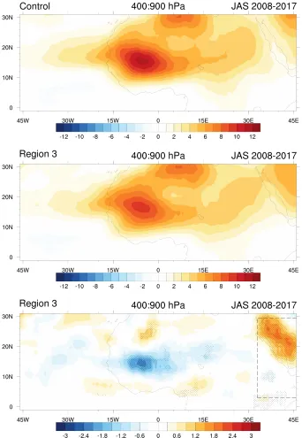
Figure 2.23 Time longitude diagram averaged over 15 to 25◦N and 400 to 900 hPa
for the 900 hPa, 20◦N, -15◦E base point regression showing baroclinic overturning (Cp k, shaded, J kg−1day−1) and EKE (contoured, starting
at 0.2 J kg−1and doubling for successive contours) for the control
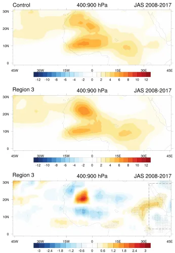
(left) and R3 simulations (middle) and the difference from the control (right). Contours in the difference plots still represent the R3 EKE. . . 50 Figure 2.24 As in Figure 2.23 but for the diabatic generation tendency (Ge) in
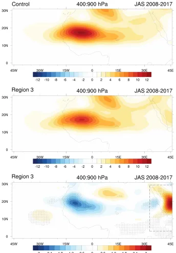
the EAPE budget for the 650 hPa, 10◦N, 0◦E base point regression. Contours still show EKE. . . 50 Figure 2.25 Time longitude diagram averaged over 5 to 15◦N and 400 to 900 hPa
for the 650 hPa, 10◦N, 0◦E base point regression showing baroclinic conversion tendencies (CA, shaded, J kg−1day−1) in the EAPE budget
and EKE (contoured, starting at 0.2 J kg−1and doubling for successive
contours) for the control (left) and R3 simulations (middle) and the difference from the control (right). Contours in the difference plots still represent the R3 EKE. . . 51 Figure 2.26 As in Fig. 2.25 but for the baroclinic conversion tendency (CA)
Figure 2.27 Control (top) and R3 (middle) barotropic conversions (CK, J kg−1
day−1) from the EKE budget averaged over JAS 2008-2017 and
ver-tically integrated over 400 to 900 hPa and the difference from the control (bottom). Stippling shows significant differences with 95% confidence. . . 52 Figure 2.28 Control (top) and R3 (middle) baroclinic overturning (Cp k, J kg−1
day−1) from the EKE budget averaged over JAS 2008-2017 and
ver-tically integrated over 400 to 900 hPa and the difference from the control (bottom). Stippling shows significant differences with 95% confidence. . . 53 Figure 2.29 Control (top) and R3 (middle) diabatic generation (Ge, J kg−1day−1)
from the EAPE budget averaged over JAS 2008-2017 and vertically integrated over 400 to 900 hPa and the difference from the control (bottom). Stippling shows significant differences with 95% confidence. 54 Figure 2.30 Control (top) and R3 (middle) baroclinic conversions (CA, J kg−1
day−1) from the EAPE budget averaged over JAS 2008-2017 and
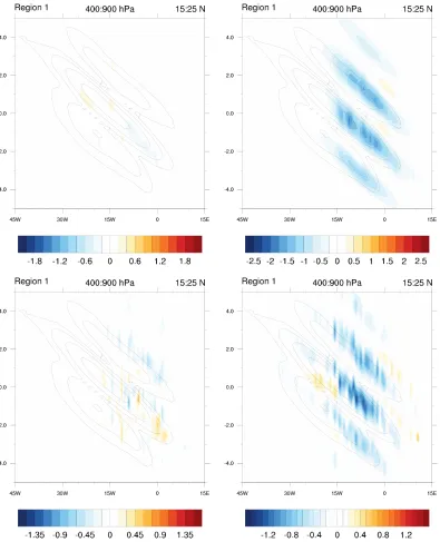
ver-tically integrated over 400 to 900 hPa and the difference from the control (bottom). Stippling shows significant differences with 95% confidence. . . 55 Figure 2.31 Time-longitude diagram showing regressed EKE (contoured, starting
at 0.2 J kg−1and doubling for successive contours) and energy budget
terms (shaded, J kg−1day−1)C
K (top left),Cp k (top right),Ge (bottom
left), andCA (bottom right) averaged over 400 to 900 hPa for the R1
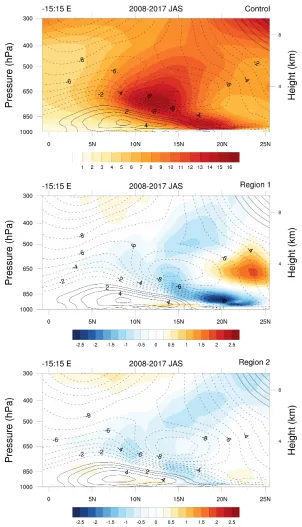
experiment simulations for the regression at the basepoint 900 hPa, 20◦N, -15◦E. . . 56 Figure 2.32 Latitude-height cross section showing the -15 to 45◦E, JAS 2008-2017
averaged EKE (J kg−1) of the control (left) and the difference of the
control from the R3 simulations (right). Contours show the averaged zonal wind every 1 m s−1with negative contours dashed. . . . 57
Figure 2.33 As in Fig. 2.32 but for the diabatic heating (K day−1). . . . 57
Figure 2.34 Latitude-height cross section showing the -15 to 15◦E, JAS 2008-2017 averaged EKE (J kg−1) of the control (top) and the difference of the
control from the R1 simulations (middle) and the R2 simulations (bottom). Contours show the averaged zonal wind every 1 m s−1with
negative contours dashed. . . 58 Figure 2.35 Latitude-height cross section showing the -15 to 15 ◦E, JAS
2008-2017 averaged diabatic heating (K day−1) of the control (top) and the
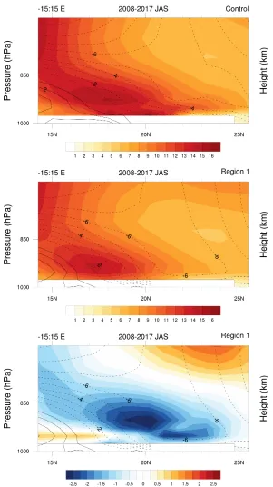
Figure 2.36 Latitude-height cross section showing the -15 to 15◦E, JAS 2008-2017 averaged EKE (J kg−1) of the control (top) and the R1 experiment
(middle) as well as the difference of the control from the R1 simu-lations (bottom). Zonal winds for are contoured every 1 m s−1with
negative contours dashed. The difference plot contouring still shows the R3 zonal winds. . . 60 Figure 3.1 Time-longitude diagram of 2-10 day filtered EKE (J kg−1) from ERAi
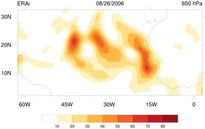
for July-August 2006. . . 86 Figure 3.2 Map of 2-10 day filtered EKE (J kg−1) from ERAi for August 26, 2006. . 87
Figure 3.3 Stabilized absolute (left) and convective (right) instability represented in thex-t plane for an easterly flow. Initially, a disturbance undergoes growth in an unstable region and disperses energy into a spreading wave packet as time increases, but then the damping begins to domi-nate the development of the wave packet and diminishes the wave packet over time. The spread of the wave packet is controlled by the total group velocityCg T of the disturbance and is bounded byCg Tmin
on the leading edge of the wave packet andCg Tmaxon the lagging edge
of the wave packet. . . 88 Figure 3.4 As in Fig. 3.3 but where the long-lived wave packet persists for
sev-eral periods despite the damping (left) and where the short-lived wave packet is diminished due to damping (right) on an stabilized absolutely unstable zonal flow. . . 88 Figure 3.5 Vertical heating profileH0(a) and vertically integrated heating (b, K
day−1) from Eq. 3.1 used in the fixed localized heating simulations. . 89
Figure 3.6 Example temperature perturbation (K) due to the heat forcing pro-vided in one time step to the model for the noise-forcing simulations. 89 Figure 3.7 Composite zonal winds (m s−1) from the average of all 775 basic states
formed over JJAS 1987-2017 atσ=0.65, roughly 650 hPa. . . 90 Figure 3.8 As in Fig. 3.7 but for the latitude-height cross section averaged over
-15 to 15◦E. . . . 90
Figure 3.9 Composite meridional PV gradient (shaded, 10−6PVU m−1) formed
from the average of all 775 basic states formed over JJAS 1987-2017 at 700 hPa. Composite zonal winds are overlaid, contoured every 2 m s−1with negative contours dashed. . . . 91
Figure 3.10 As in Fig. 3.9, but for the latitude-height cross section averaged from -15 to 15◦E. . . . 91
Figure 3.11 Streamfunction (contoured every 0.5×10⁵m2s−1with negative
Figure 3.12 Averaged EKE (shaded, J kg−1) from perturbation horizontal winds
atσ=0.65 (top) andσ=0.95 averaged over days 5 through 15 of simulation using the JJAS 1987-2017 composite basic state. Zonal winds from the basic state are contoured every 1 m s−1with negative
contours dashed. The black dot represents the location of the initial heating perturbation. . . 93 Figure 3.13 As in Fig. 3.12 but for the latitude-height cross section averaged over
-15 to 15◦E. . . . 93
Figure 3.14 Time-longitude diagram of EKE (J kg−1) atσ=0.85 resulting from
fixed-heating on the JJAS 1987-2017 composite basic state averaged over 5 to 20◦N. The black dot represents the location of the initial
heating perturbation. . . 94 Figure 3.15 As in Fig. 3.14 but for the quantityα. The horizontal line at day 20
marks the cut-off for short-lived wave packet classification. . . 94 Figure 3.16 Streamfunction (contoured every 0.5×10⁵m2s−1with negative
con-tours dashed) atσ=0.85 resulting from fixed-heating initiation on the THK basic state for days (from top to bottom) 5, 11, 17, and 90. . 95 Figure 3.17 Time-longitude diagram of EKE (J kg−1) atσ=0.85 resulting from
fixed-heating on the THK basic state averaged over 5 to 20◦N. The black dot represents the location of the initial heating perturbation. 96 Figure 3.18 As in Fig. 3.17 but for the quantityα. The horizontal line at day 20
marks the cut-off for short-lived wave packet classification. . . 96 Figure 3.19 Basic state zonal winds (m s−1) atσ=0.65 for the short-lived (top),
intermediate-lived (middle), and long-lived (bottom) composites. The black dot shows the location of the initial heating perturbation. 97 Figure 3.20 Difference from the climatological JJAS 1987-2017 basic state zonal
winds (m s−1) atσ=0.65 for the short-lived (top), intermediate-lived
(middle), and long-lived (bottom) composites. The climatological basic state zonal winds are contoured every 1 m s−1with negative
contours dashed. . . 98 Figure 3.21 Latitude-height cross section of the basic state zonal winds (m s−1)
averaged over -15 to 15◦E for the short-lived (top), intermediate-lived
(middle), and long-lived (bottom) composites. . . 99 Figure 3.22 Latitude height cross section of the difference from the climatological
JJAS 1987-2017 basic state zonal winds (m s−1) averaged over -15 to
15◦E for the short-lived (top), intermediate-lived (middle), and
long-lived (bottom) composites. The climatological basic state zonal winds are contoured every 1 m s−1with negative contours dashed. . . 100
Figure 3.23 Meridional PV gradient (shaded, 10−6PVU m−1) at 700 hPa for the
short-lived (top), intermediate-lived (middle), and long-lived (bot-tom) composites. Zonal winds are contoured every 2 m s−1with
Figure 3.24 Latitude-height cross section of the meridional PV gradient (shaded, 10−6PVU m−1) averaged from -15 to 15◦E for the short-lived (top),
intermediate-lived (middle), and long-lived (bottom) composites. Zonal winds are contoured every 2 m s−1 with negative contours
dashed. . . 102 Figure 3.25 Streamfunction at days 5 (top), 11 (middle), and 17 (bottom),
sepa-rated by roughly one AEW period, initiated by a fixed-heating anomaly on the short-lived composite basic state. Contours are separated ev-ery 0.5×10⁵m2s−1. . . 103
Figure 3.26 As in Fig. 3.25 but at day 32 and with a contour interval of 2500 m2s−1103
Figure 3.27 Streamfunction at days (from top to bottom) 5, 11, 17, and 32 initiated by a fixed-heating anomaly on the intermediate-lived composite basic state. Contours are separated every 0.5×10⁵m2s−1. . . 104
Figure 3.28 Streamfunction at days (from top to bottom) 5, 11, and 17 initiated by a fixed-heating anomaly on the long-lived composite basic state. Contours are separated every 0.5×10⁵m2s−1. . . 105
Figure 3.29 As in Fig. 3.28 but for day 32. Contours are separated every 105m2s−1.105
Figure 3.30 Maps of EKE (J kg−1) averaged from days 5 through 15 forσ=0.65
(left) andσ=0.95 (right), resulting from the fixed-heating anomaly on the (from top to bottom) SL, IL, and LL composite basic states. The basic state zonal winds are contoured every 1 m s−1with negative
contours dashed. . . 106 Figure 3.31 Latitude-height cross section of EKE (J kg−1) averaged from over -15
to 15◦E and over days 5 through 15 resulting from the fixed-heating
anomaly on the (from top to bottom) SL, IL, and LL composite basic states. The basic state zonal winds are contoured every 1 m s−1with
negative contours dashed. . . 107 Figure 3.32 Time-series of the globally averaged EKE (J kg−1) resulting from the
fixed-heating anomaly on the SL, IL, and LL basic states. . . 108 Figure 3.33 Time-series of the globally averaged EKE growth rates (day −1)
re-sulting from the fixed-heating anomaly on the SL, IL, and LL basic states. The mean growth rate, averaged over the last 50 days of the simulation, is shown by the dashed line. . . 108 Figure 3.34 Time-longitude diagram of EKE (J kg−1) atσ=0.85 resulting from
fixed-heating on the short-lived (left, days 1 through 15), intermediate-lived (middle, days 1 through 35), and long-intermediate-lived (right, days 1 through 100) composite basic states averaged over 5 to 20◦N. The black dot represents the location of the initial heating perturbation. The con-tour on the long-lived figure shows the 0.25 J kg−1contour for direct
comparison to the values in the short- and intermediate-lived simu-lations. . . 109 Figure 3.35 As in Fig. 3.34 but for the quantityα. The horizontal line at day 20
Figure 3.36 Total group velocity (m s−1) averaged over days 30 through 35 of the
simulation for the climatological (top left), SL (top right), IL (bottom left), and LL (bottom right) composite basic states.Cg T is evaluated
from Eq. 3.4, integrated over half-wavelengths in the zonal direction, from -5 to 30◦N meridionally, throughout the model depth in the
vertical direction. . . 110 Figure 3.37 Total group velocity (m s−1) averaged over days 30 through 35 of the
simulation for the SL (top), IL (middle), and LL (bottom) composite basic states shown by the blue line.Cg T is evaluated from Eq. 3.4,
integrated over six gridpoints in the zonal direction, from -5 to 30◦N meridionally, throughout the model depth in the vertical direction. The dashed blue line shows the window of plus or minus one standard deviation from the mean total group velocity. For comparison, the black line in each plot is the same total group velocity shown in Fig. 3.36.111 Figure 3.38 Maps forσ=0.85 showing the geopotential flux convergence (shaded,
J kg−1s−1), and ageostrophic geopotential flux vectors (m3s3) for the
wave packet resulting from the fixed-heating anomaly on the (from top to bottom) SL, IL, and LL composite basic state at day 7.5. EKE is contoured starting at 0.01 J kg−1and doubling for each successive
contour. . . 112 Figure 3.39 Streamfunction at days (from top to bottom) 5, 11, and 17 initiated
by a fixed-heating anomaly on the basic state formed the a 15 day average centered around August 15, 1995. Contours are separated every 0.5×10⁵m2s−1. . . 113
Figure 3.40 As in Fig. 3.39 but for day 39 with contours separated every 1000 m2s−1.113
Figure 3.41 Streamfunction at days (from top to bottom) 5, 11, and 17 initiated by a fixed-heating anomaly on the basic state formed the a 15 day average centered around September 4, 2006. Contours are separated every 0.5×10⁵m2s−1. . . 114
Figure 3.42 As in Fig. 3.41 but for day 28 with contours separated every 4000 m2s−1.114
Figure 3.43 Time-longitude diagram ofαatσ=0.85 resulting from fixed-heating on the August 15, 1995 basic state (left) and the September 4, 2006 (right) basic state averaged over 5 to 20◦N. The black dot represents
the location of the initial heating perturbation. . . 115 Figure 3.44 Total group velocity (m s−1) averaged over days 15 through 20 of the
simulation for the August 15, 1995 basic state (left) and the September 4, 2006 (right) basic state simulations.Cg T is evaluated from Eq. 3.4,
integrated over half-wavelengths in the zonal direction, from -5 to 30
◦N meridionally, throughout the model depth in the vertical direction.115
Figure 3.45 Maps of zonal winds (m s−1) at σ =0.65 for the 15 day averaged
Figure 3.46 Maps of meridional PV gradient (10−6PVU m−1) atσ=0.65 for the 15
day averaged basic states centered around August 15, 1995 (top) and September 4, 2006 (bottom). Contours show the zonal winds every 2 m s−1of the basic states, with negative contours dashed. . . 117
Figure 3.47 Latitude-height cross section of zonal winds (m s−1) averaged over -15
to 15◦E for the 15 day averaged basic states centered around August
15, 1995 (top) and September 4, 2006 (bottom). The black dot shows the location of the initial heating perturbation. . . 118 Figure 3.48 Latitude-height cross section of meridional PV gradient (10−6PVU
m−1) averaged over -15 to 15◦E for the 15 day averaged basic states
centered around August 15, 1995 (top) and September 4, 2006 (bot-tom). Contours show the zonal winds every 2 m s−1of the basic states,
with negative contours dashed. . . 118 Figure 3.49 Time-longitude diagram of EKE (J kg−1) atσ=0.85 averaged over 5
to 20◦N resulting from noise-forcing for the climatological (top left),
SL (top right), IL (bottom left), and LL (bottom right) composite basic states. . . 119 Figure 3.50 Maps of EKE (J kg−1) averaged from days 5 through 15 forσ=0.65
(left) andσ=0.95 (right), resulting from the noise-forcing on the (from top to bottom) climatological, SL, IL, and LL composite basic states. The basic state zonal winds are contoured every 1 m s−1with
negative contours dashed. . . 120 Figure 3.51 Zonal wavenumber frequency spectra of the meridional winds at
σ=0.85 resulting from the noise-forcing and tapered to 10% using a split-cosine-bell tapering outside of the AEW stormtrack region from -60 to 50◦E and 5 to 25◦N for the climatological (top left), SL (top
right), IL (bottom left), LL (bottom right) composite basic states. . . . 121 Figure 3.52 Zonal wavenumber frequency spectra of the meridional winds at
σ=0.85 resulting from the fixed-heating anomaly and tapered to 10% using a split-cosine-bell tapering outside of the AEW stormtrack region from -60 to 50◦E and 5 to 25◦N for the climatological (top left), SL (top right), IL (bottom left), LL (bottom right) composite basic states.122 Figure 3.53 Number of basic states that produced wave packets produced from
the fixed-heating categorized as SL (blue), IL (green), and LL (red) for each month from the full set of 775 basic states. . . 123 Figure 3.54 JJAS time-series of 1987-2017 averaged EKE (J kg−1) at 650 hPa
CHAPTER
1
INTRODUCTION
1.1
Definitions
African easterly waves (AEWs) are the dominant synoptic feature of the summer West African monsoon (WAM). These disturbances propagate westward across northern tropical Africa and across the Atlantic Ocean with wavelengths of approximately 3000-4000 km and periods of about 2-10 days (e.g., Burpee 1972). They occur during the northern hemisphere warm season (June - October) with peak activity in July and August. They follow two distinct paths; a northern track centered about 20◦N, and a southern track centered about 10◦N.
dynamics (Diedhiou et al. 1999, 2002).
1.2
Motivations
AEWs have a broad impact in the northern hemisphere tropics. While AEWs propagate across northern Africa, they are associated with strong variability of precipitation (e.g. Reed et al. 1977; Mekonnen et al. 2006; Laing et al. 2008). As such, studies that improve upon the understanding of AEWs aid in forecasting for the region. AEWs are also the source of a majority of North Atlantic tropical cyclones (e.g. Avila and Pasch 1992; Russell et al. 2017), so they also hold significance for countries in the Caribbean and North America. Furthermore, AEWs can occasionally propagate into the North Pacific where they play a role in the genesis of Pacific easterly waves and tropical cyclones (e.g., Molinari et al. 1997; Rydbeck et al. 2017), spreading their influence to communities in the Pacific Islands and East Asia.
A large body of literature has described an association between AEWs and organized patterns of precipitation, mainly through mesoscale convective systems (MCSs). Reed et al. (1977) formed a composite wave structure using observations from Phase III of the Global Atmospheric Research Program (GARP) Atlantic Tropical Experiment (GATE), and their composite showed strong convection ahead of AEW troughs in West Africa. Fink and Reiner (2003) found that 42% of MCSs in the Sahel are forced by AEWs where the primary role of the AEW is to initiate and organize the MCSs. Similarly, Mekonnen et al. (2006) used temporal spectral analysis to show that convection on the AEW time scale, 2-6 days, accounts for 25% to 35% of the total variance for convection across this region. More recent work by Russell (2018) concludes that convection helps maintain and propagate AEWs and that AEWs further help maintain MCSs in a positive feedback loop, analogous to the stratiform instability proposed by Mapes (2000). Given the relationship between AEWs and MCSs, AEWs have a strong impact on the West African population.
Irma, and Maria during the 2017 hurricane season. Each of these storms caused substantial damage and loss of life in the Caribbean Islands and United States.
It has also been found that AEWs can reinvorgate as easterly waves over the Pacific Ocean (e.g. Avila and Pasch 1992). Molinari et al. (1997) showed the existence of a meridional potential vorticity (PV) gradient sign reversal during the summer of 1991 near 700 hPa over the Caribbean Sea, leading to the speculation that AEWs could strengthen in this region or that new easterly waves could generate over the Caribbean. More recent studies have shown that these Pacific easterly waves can formin situover the Pacific rather than originating
solelyfrom AEWs propagating across the Caribbean Sea (e.g. Serra et al. 2008; Rydbeck et al. 2017). While this indicates that AEWs are not the only source of disturbances that form these disturbances, it is still evident that AEWs that propagate beyond the Caribbean have the potential to lead to enhanced easterly wave activity over the Pacific basin.
1.3
Background
1.3.1
Early Understanding
The earliest descriptions of AEWs in the published scientific literature include Piersig (1936) who examined surface pressure variations along the West African coast and Regula (1936) who categorized them as a class of unique cyclonic disturbances off the coast of Africa. From West African coastal and Cape Verde Island stations, Regula (1936) discovered surface pressure oscillations spanning from the Monrovia station around 6◦N up to the Rio de Oro
station around 24◦N with a period of about 4 days, and a perturbation amplitude of about
the low-pressure anomaly of the wave. He tracked these disturbances over West Africa using daily pressure maps, tracing their origin to the vicinity of the Hoggar Mountains. From this tracking, Hubert suggested that the hurricane that hit Long Island, NY on 21 September, 1938 began as an AEW.
Carlson (1969) proposed that AEWs originate from squall lines that formed over elevated terrain in East Africa, while Frank (1970) hypothesized that AEWs result from a mechanical forcing effect due to flow over this elevated terrain. Burpee (1972) presented evidence that the AEJ is associated with a reversal in the meridional gradient of PV, satisfying the Charney-Stern necessary condition for mixed baroclinic-barotropic instability (Charney and Charney-Stern 1962), and concluded that AEWS are a result of disturbances growing in this unstable region. For decades, this dry hydrodynamic instability mechanism was the paradigm for the mechanism for AEW development.
Fig. 1.1 shows the June-October (JJASO, abbreviated for each month in the date range), 1987-2017 time-mean zonal winds from the Interim European Center for Medium-Range Weather Forecasts (ECMWF) Reanalysis (ERAi) data set. Fig. 1.1a shows the climatological zonal winds at 650 hPa, the approximate level of the AEJ core. It lies between about 5 and 20◦N and extends from East Africa, just east of 45◦E, to west of the western coast of Africa
over the Atlantic Ocean. A latitude-height cross section of the zonal winds zonally averaged from -15 to 15◦E is shown in Fig. 1.1b. The winds in the peak of the climatological AEJ reach about 12 m s−1at 650 hPa, and just below the AEJ are the surface westerlies from the WAM during the summer, ranging from about 1 to 2 m s−1, and causing enhanced vertical shear
associated with the AEJ.
Also shown in Fig. 1.1 are the meridional PV gradient at 650 hPa (Fig. 1.1c) and the same latitude-height cross section (Fig. 1.1d). The PV gradient sign reversal that Burpee (1972) first observed is well defined along much of the longitudinal extent of the AEJ, exhibiting a meridional reversal just near and below the AEJ core and a vertical reversal above and below the AEJ. The horizontal and vertical PV gradient reversal shown here permits both barotropic and baroclinic development.
The results of Burpee (1972) promoted the paradigm that AEWs are the result of small amplitude disturbances growing on the unstable AEJ. This was confirmed by studies that examined observed energetics of AEWs (e.g., Reed et al. 1977) and by modelling studies that showed the most unstable normal mode of an idealized AEJ resemble observed AEWs (e.g., Rennick 1976; Simmons 1977; Thorncroft and Hoskins 1994).
(a) (b)
(c) (d)
Figure 1.1: ERAi June-October, 1987-2017 averaged zonal winds (shaded, m s−1, in a,b)
map at 650 hPa (a) and latitude-height cross section averaged over -15 to 15◦E (b) and meridional PV gradient (shaded, PVU 1000 km−1, in c,d) map at 650 hPa (c) and
latitude-height cross section averaged over -15 to 15◦E (d). For comparison, zonal winds are overlaid
(contoured every 1 m s−1) in (c) and (d), with dashed lines indicating easterly flow. Winds less than 6 m s−1are drawn with thicker markings to highlight the AEJ.
equatorward side (e.g., Thorncroft and Hodges 2001). A good index for AEW activity is eddy kinetic energy (EKE). EKE is defined as
Ke=
1
2V~0·V~0 (1.1)
whereV~0=u0iˆ+v0jˆis the perturbation horizontal flow velocity. To specifically highlight the AEW activity, a band pass frequency filter is typically applied toV~0on the AEW time
scale. Fig. 1.2 shows the 2-10 day filtered EKE averaged over JJASO, 1987-2017. The southern track is located roughly at the level of the peak AEJ (650 hPa) and is shown in Fig. 1.2a. The southern track follows along the southern flank of the AEJ, beginning as far back as roughly 40◦E, and it peaks just downstream of the AEJ core near roughly 20◦E. Meanwhile, the
zonally along the AEJ as the southern track does but is instead more localized over West Africa.
Shown in Fig. 1.2c is a latitude-height cross section of EKE averaged across -15 to 15
◦E. Comparing this to Fig. 1.1d, the southern track lies in a region of horizontal meridional
PV gradient reversal, implying that disturbances in the southern track develop primarily due to barotropic energy conversions. Additionally, the northern track lies in a region of vertical meridional PV gradient reversal, implying that disturbances in the northern track develop primarily due to baroclinic energy conversions. The energetics of AEWs in both of these tracks have been presented in previous literature, and barotropic tendencies indeed dominate in the southern track, while baroclinic tendencies dominate in the northern track (Céron and Guérémy 1999; Pytharoulis and Thorncroft 1999).
(a) (b)
(c)
Figure 1.2: ERAi June-October, 1987-2017 averaged EKE (shaded, J kg−1) map at 650 hPa
(a) and 925 hPa (b) and latitude-height cross section averaged over -15 to 15◦E (c). As in
Figure 1.1, zonal winds (contoured every 1 m s−1) at 650 hPa are overlaid in (a,b) and from
the -15 to 15◦E average in (c).
energy conversions, but the growth rates of AEWs drop drastically west of 30◦W (Thorncroft and Hoskins 1994). Additionally, in this merged part of the AEW stormtrack, the waves are more nonlinear in nature, while the waves over the land are more linear (Thorncroft 1995).
1.3.2
Recent Developments
Although the consensus was reached that AEWs originate from the development of small amplitude disturbances along an unstable AEJ, more recent studies have indicated that this hydrodynamic instability of the AEJ alone cannot account for the observed growth rates seen in AEWs (e.g., Hall et al. 2006; Hsieh and Cook 2008). Hall et al. (2006) demonstrated in an idealized model that moderate low-level damping in the lower levels (representative of turbulent transfer of heat and momentum with the surface) was sufficient to reduce the growth rate of AEWs to nearly zero, stabilizing the AEJ. As a result, they concluded that AEWs cannot be the result of small amplitude disturbances growing on an unstable AEJ; either the growth rates must be higher than dry linear modeling indicates or the initial disturbances must be larger.
Within the past decade, some candidates for mechanisms responsible for the larger observed growth rates in AEWs have been proposed. One such mechanism is a destabiliza-tion caused by dust-radiative effects (Grogan et al. 2016). AEWs are known to contribute to episodic synoptic scale plumes of Saharan mineral dust (SMD) aerosols (Knippertz and Todd 2010). As they interact with their surroundings, these plumes can modulate properties of the atmosphere to change the energetics and therefore dynamics of the local distur-bances, either through a direct radiative effect or an indirect microphysical effect (Zhu et al. 2007). In their study, Grogan et al. (2016) used a dust-coupled version of the Weather Research and Forecasting model (WRF) to examine the direct radiative effect of SMD on AEW growth rates. They found that waves in the presence of dust had substantially larger growth rates, with growth rates ranging from around 5 to 20% larger. These larger growth rates are attributed to an increase of the barotropic and baroclinic conversion rates in the AEWs as a direct result of dust-radiative feedback. Nathan et al. (2017) further showed in an idealized dust-coupled WRF simulation that in the case of an AEJ that was sub-critical to AEWs, the AEWs were still destabilized in the presence of SMD; therefore, they concluded that this destabilizing effect may offset the neutralization of such low-level damping from Hall et al. (2006).
the PV gradient reversal over the Sahel (Thorncroft and Blackburn 1999) and therefore to the barotropic and baroclinic conversions in the AEWs (Hsieh and Cook 2005, 2007). This is already included in the JJAS, 1968-1998 climatological basic state from Hall et al. (2006); however, such a long term average as in Hall et al. (2006) could have the effect of smearing out the PV gradient and could therefore lead to the lower growth rates in their simulation. Leroux and Hall (2009) used the same model to simulate AEWs as Hall et al. (2006), but they used many separate ten day averages spanning the northern hemisphere summer months of several years. Their ten day averaged basic states would not suffer from this smearing effect, yet still the growth rates from their strongest AEWs were too small compared to observed AEWs. Therefore, if convection plays a role in the the growth of AEWs, it is likely not solely due the long-term role of the ITCZ convective destabilization, but on the smaller scale of the waves themselves as a result of individual AEWs coupling with convective systems.
In a case study, Berry and Thorncroft (2005) tracked the AEW that later formed Hurricane Alberto (2000) and concluded that convection directly led to a downstream anomalous PV maxima that promoted the propagation and maintenance of the AEW. Extending this work, Berry and Thorncroft (2012) demonstrated through the energetics of a simulated AEW that diabatic heating associated with convection in the AEW is as important as the adiabatic processes in wave development. They concluded that moist convection serves to directly enhance the magnitude of PV anomaly associated with the AEW, promoting the Diabatic Rossby Wave mechanism first proposed by Parker and Thorpe (1995) for mid-latitude baroclinic eddies. Additionally, Russell (2018) showed that MCSs in the vicinity of the AEW helps both to propagate and grow the AEW and that AEWs in turn also help maintain the MCSs. Russell (2018) showed that the superposition of coupled moist PV anomalies from the MCSs with the barotropically developing dry PV anomalies from the AEWs enhances the growth of southern track AEWs in a manner similar to the stratiform instability mechanism (Mapes 2000). Russell also demonstrated that deep moist convection helps to maintain the AEW PV column against the background shear. These results imply that moist processes may explain at least some of the higher growth rates needed to overcome the stabilization of low-level damping.
large enough to overcome low-level damping as shown in Hall et al. (2006), AEWs will not grow over time but will instead remain as the slowest-decaying mode resulting from an initial disturbance. This “triggering hypothesis” seems to be the current consensus for the dominant mechanism responsible for AEW formation. The success of large amplitude triggers in forming AEWs was first shown in Thorncroft et al. (2008). They used the same model with a fixed climatological basic state as in Hall et al. (2006), but they initiated the model with a localized heating anomaly representative of the latent heat release from a large MCS near the entrance region of the AEJ near the Darfur Mountains. This anomalous heating was prescribed in the model for only the first 24 hours. As a result of this initial heating, a baroclinic vortex formed and was advected eastward into the region of the PV gradient reversal along the AEJ. There, the anomaly began to develop and resemble an AEW. By keeping the basic state fixed, the initial anomaly was free to extract energy from the AEJ without diminishing the AEJ, and by day 11 of their simulation, a series of AEWs had developed. The low-level damping used in the model was enough to stabilize the AEJ, but a series of AEWs still emerged from their initial disturbance. Because of this damping, rather than the fastest growing normal mode, it was the slowest decaying normal mode that led to the development of consecutive AEWs. The authors therefore conclude that a large MCS will lead to an AEW roughly five days later, followed by a series of three or four AEWs.
This triggering hypothesis has since gained a lot of traction as a mechanism for AEW genesis. Leroux and Hall (2009) used their ten day averages in the same model with fixed basic states to examine the response to the same MCS heating as Thorncroft et al. (2008), showing a variety of AEW responses. Their results led them to support the conclusions of Hall et al. (2006) that small, isolated disturbances cannot develop on the AEJ into observed AEWs. They also found that some variations of the AEJ would not support a slowest decaying normal mode representative of AEWs, and most (by far) of those that did so were classified in their study as weak. By compositing their ten day basic states based on the strongest AEW responses, they also found that a strong AEW response requires a broad, strong AEJ with underlying surface monsoon westerlies.
Triggers need not only be convective in nature. In another study, Leroux et al. (2011) again used the same model as Thorncroft et al. (2008), only this time they allowed the basic state to evolve over time in order to show that disturbances from the North Atlantic mid-latitude stormtrack could play the role of large amplitude precursors for AEWs at least as well as convective triggering events. Their results even provided intermittency that closely resembled the observed intermittency of AEW activity, a problem that convective triggers, with the persistent ITCZ exhibiting diurnal convection (e.g., Laing et al. 2008), fails to fully explain.
Diaz and Aiyyer (2013a,b) offer an alternative mechanism for AEW genesis; upstream development from previously existing AEWs. In their first study, Diaz and Aiyyer (2013a) constructed an eddy kinetic energy budget for a composite AEW and concluded that AEWs exhibit upstream energy dispersion. With this upstream energy dispersion, energy propa-gates eastward, providing a source of energy for the development of a new, consecutive AEW upstream as part of a series of AEWs. Diaz and Aiyyer (2013b) then used their eddy kinetic energy budget for a case study, the AEW that led to Hurricane Alberto (2000), to show that this wave owed its genesis to the upstream energy dispersion of a previous wave, verifying that upstream development is indeed a valid genesis mechanism for AEWs. However, the question then is, if waves can be formed by a previous AEW, and since AEWs do not occur continuously throughout a given season, what leads to the genesis of the first wave in a series of consecutive AEWs? It is likely that AEWs are continuously forced by variety of mechanisms, including linear normal mode instability and finite amplitude precursors that are ubiquitous in nature. An implication of the results by Diaz and Aiyyer (2015) is that the instability involved should be viewed, not from the perspective of only temporal growth but rather also of spatial growth. This is further explored in this study.
1.3.3
Local instability
and Charney (1947) were the first to describe the synoptic baroclinic eddies responsible for most of the weather in the mid-latitudes. They both used simplified atmospheric models to demonstrate that the fastest growing disturbances growing in a zonally homogenous, baroclinically unstable flow closely resemble the structure of observed perturbations.
Theoretical treatment of aforementioned instabilities are usually based on plane par-allel, zonally uniform jets. However, for the AEJ-AEW system, the region of instability is localized along the zonal extent, as shown in Fig. 1.1c. The region of PV-gradient reversal occurs only over a few AEW wavelengths. Thus, a single AEW can only experience barotropic and baroclinic conversions for a limited time before it propagates westward out of the un-stable region. Past studies have examined the impact of such localized regions of instability in idealized flow regimes (e.g., Pierrehumbert 1984; Huerre and Monkewitz 1990), demon-strating a non-trivial perturbation response to localized instability. For this local instability (orspatialinstability), both temporal and spatial growth play a role in the development of instabilities. Local instability can be classified as either “absolute” or “convective” instability, so named from their relevance in plasma physics (Briggs 1964). This delineation arises due to two possibilities:
1. A developing, dispersive wave packet grows and spreads within an unstable region. As the wave packet spreads upstream and downstream, individual waves propagate downstream, but new waves form upstream via upstream dispersion, and these new waves reemerge in the unstable region, continuing the process while some part of the wave packet always remains in the unstable region. A fixed point in the domain is eventually characterized by exponential growth. This is the case for absolute instability. This process is represented conceptually for easterly flow in the left figure of Fig. 1.3.
2. A developing wave packet will undergosomeinitial growth while it is in the localized unstable region, but before the wave packet can spread and grow substantially, the waves are advected out of the region of instability. A fixed point in the domain will see growth for limited time followed by decay. This is the case for convective instability. This process is shown conceptually for easterly flow in the right figure of Fig. 1.3. Once the waves have left the unstable region, growth of the wave packet will cease and the developments will be susceptible to damping.
Figure 1.3: Absolute (left) and convective (right) instability represented in thex-t plane for an unstable easterly flow. Initially, a disturbance undergoes growth in an unstable region and disperses energy into a spreading wave packet as time increases. The spread of the wave packet is controlled by the total group velocityCg T of the disturbance and is bounded
byCg Tmin on the leading edge of the wave packet andCg Tmaxon the lagging edge of the wave
packet. IfCg T = 0 falls within this cone, then there is both upstreamand downstream
development in the wave packet, and the flow is absolutely unstable. Otherwise, the flow is convectively unstable. Adapted from Diaz and Aiyyer (2015).
instability was first introduced to the atmospheric sciences in an effort to understand the localization of the mid-latitude stormtracks. However, it was shown that these baroclinic eddies are only convectively unstable as they disperse most of their energy downstream (e.g., Simmons 1977; Swanson and Pierrehumbert 1994). Since then, local instability has not been the subject of many studies in the field.
exhibits intraseasonal variability and experiences nonlinear impacts of AEWs growing at the expense of the AEJ. Additionally, observed AEWs have intermittent periods of activity which was not captured in their simulation. Nevertheless, this study demonstrates that the observed AEJ may at least occasionally support absolute instabilities. A further implication of this study is that, so long as the AEJ is absolutely unstable, small disturbancescandevelop into observed AEWs, counter to the conclusions of previous studies (e.g. Hall et al. 2006; Thorncroft et al. 2008). Although it will take substantially longer than the 11 day simulation by Thorncroft et al. (2008), if the AEJ is absolutely unstable, small disturbances may still develop instabilities as a packet of AEWs as shown by Diaz and Aiyyer (2015), and they may continue to develop locally until the waves reach the amplitude of observed AEWs, provided the AEJ remains absolutely unstable throughout the entirety of this evolution.
Diaz and Aiyyer (2015) used the total group velocity,Cg T, from Orlanski and Chang (1993)
to determine if the instability exhibited in their simulation was an absolute or convective instability, where
Cg T
min<0< Cg T
max⇒absolute instability, and
Cg T
min< Cg T
max<0⇒convective instability.
(1.2)
Cg T can be interpreted as the velocity that the wave packet translates due to advection from
the flow and from ageostrophic flux, the term responsible for upstream development. More plainly, the conditions above state that if the leading edge of the wave moves downstream while the lagging edge moves upstream, then the wave packet is an absolute instability, where if both the leading and lagging edge of the packet are moving downstream, the wave packet is a convective instability. Convective instability could also occur if the total group velocity is everywherepositive, so we can also have the case
0< Cg T
min< Cg T
max⇒convective instability,
following the leading edge of the wave packet and(Cg T)maxis the eastern-most red line
following the lagging edge of the wave packet. By using this quantity, Diaz and Aiyyer (2015) showed that the total group velocity satisfied the absolute instability criteria in Eq. 1.2 for the climatological AEJ; however, since the AEJ varies intraseasonally, this may not always be the case. More work is needed to determine to what extent absolute instability can explain AEW activity.
1.4
Research Objectives and Scientific Questions
Diaz and Aiyyer (2015) demonstrated that the climatological AEJ is absolutely unstable, yet we rarely see periods of extensively long-lived AEW activity. It may be that the climatologi-calAEJ is absolutely unstable, but not the typical AEJ on which observed AEWs develop. Additionally, studies have linked AEW activity to regions of elevated terrain (Berry and Thorncroft 2005; Mekonnen et al. 2006), but it is not yet clear what role orography plays in the AEW life cycle. These are gaps in knowledge regarding AEW dynamics that we hope to help fill. In this dissertation, we seek to answer the two following questions:
1. To what extent do the prominent orographic features over Africa impact the structure and intensity of the AEW stormtrack?
2. How does the absolute instability of the AEJ vary intraseasonally, and how does this variation effect the lifetime of AEW wave packets?
To answer these questions, we implement a variety of tools and data. We use the Weather Research and Forecasting model (WRF, Skamarock et al. 2008) to perform simulations investigating the sensitivity of AEW activity to north African topography. We also make use of the same model employed in Hall et al. (2006) and Thorncroft et al. (2008). This model is an adiabatic, primitive equation model, fully described in Simmons and Hoskins (1976). Like Thorncroft et al. (2008), we implement this model using an idealized configuration with a fixed background flow and an initial trigger.
For comparison of results as well as for initial and boundary conditions in the WRF model, we use the ECMWF Reanalysis-Interim (ERAi, Dee et al. 2011). ERAi has a horizontal resolution of T255 (0.70◦near the equator) and 60 vertical levels. To compare the
data is interpolated to daily means on a 2.5 by 2.5◦global grid. Additionally, WRF uses the United States Geological Survey (USGS) Global Multi-resolution Terrain Elevation Data 2010 (GMTED2010) for its topography data (Danielson and Gesch 2011). The 30-arc-second USGS GMTED2010 elevation data is used to interpolate to 10-arc-minute elevation data to be used as the default input for numerical simulations in WRF. Lastly, we use the National Centers for Environmental Prediction-2 reanalysis (NCEP2, Kanamitsu et al. 2002) to form the various background flows used as input in our idealized simulations where we initiate perturbations with an initial trigger as in Thorncroft et al. (2008). The NCEP2 reanalysis data has a horizontal resolution of T62 (1.9◦ near the equator), 28 vertical levels, and is
CHAPTER
2
THE IMPACT OF OROGRAPHY ON THE
SIMULATED AFRICAN EASTERLY WAVE
STORMTRACK
2.1
Background
Figure 2.1 shows the southern and northern AEW stormtracks at 650 and 925 hPa respec-tively. The stormtrack is represented by JAS 2008-2017 averaged EKE calculated from 2-10 day band-pass filtered ERAi horizontal winds. In both panels, the contours show surface elevation using USGS GMTED2010 data.
Along both the southern and northern AEW stormtracks, the surface is defined by pronounced orographic features. The southern track begins just west of the Ethiopian highlands located at roughly 40◦E. The Darfur mountains lie downstream along the
south-ern track at around 25◦E, followed by the Jos plateau and Cameroon highlands near 12 ◦E, and just near the Atlantic coast at -10◦E are the Guinea highlands. To the north along
in Chapter 1, numerous prior studies have suggested that elevated terrain over Africa are instrumental in the origin or amplification of AEWs. The goal of this study is to determine to what extent, if any, these regions of elevated terrain impact the two stormtracks.
Figure 2.2 shows the JAS 2008-2017 time mean of outgoing longwave radiation (OLR) with surface elevation contours. The intertropical convergence zone (ITCZ) is clearly high-lighted by the zonally extending band of low OLR values, centered roughly around 10◦N.
Along the ITCZ, local minima of OLR are coincident with areas of pronounced orography, indicating a connection between moist convection and enhanced topography. Indeed, convection tends to initiate on the leeward side of these areas of high terrain, likely as a result of thermal forcing from elevated heat sources (e.g., Laing et al. 2008; Hodges and Thorncroft 1997) and orographic forcing from the surface westerly flow over the terrain. Many studies have tied the origin of AEWs to these regions of elevated terrain through various mechanisms. Carlson (1969) concluded that these disturbances originate in east-ern Africa with possible initiation connected to the convective processes associated with the mountains. Within the limited data network used in his study, Carlson suggested the Cameroon mountains as a favorable wave initiation site.
Mekonnen et al. (2006) further examined the association between convection and AEWs by using satellite derived cloud brightness temperature and reanalysis data sets. From spectral analysis of the cloud brightness temperature, they showed that across all of tropical North Africa, 2-6 day (the time scale of AEWs) filtered cloud brightness temperature variance is of similar magnitude, and that within the regions of deep convection, this time-scale accounts for about 25% - 35% of the total variance. They then compared this result to variances of dynamical quantities filtered on this same 2-6 day time scale, showing marked differences between eastern and western Africa. The variances of these fields are strongest west of 10◦E and are much weaker eastward. They concluded that convection generated
on the westward side of east African mountains near Darfur and Ethiopia play a role in AEW initiation. Their results supported the notion of convection as AEW triggers, with the Darfur mountains being the more substantial source for initiation.
formed. They argue that it is the merging of these smaller PV maxima that assist AEWs to undergo tropical cyclogenesis. These results regarding convective initiation support the findings of Mekonnen et al. (2006), pointing again to the role of orography in providing a source for convective triggers for AEW development. Additionally, these results emphasize the role of orography in AEW development further downstream and in tropical cyclogensis.
Lin et al. (2005) also examined the pre-Alberto AEW and similarly found a connection between the AEW, convection, and orography by using satellite imagery to trace the dis-turbance all the way back to an MCS that formed on the leeward side of the Ethiopian highlands. They found the availability of water vapor to be a limiting factor for moist con-vection embedded in the pre-Alberto AEW, and that the presence of topography modulated the MCSs within the disturbance through regulation of the available water vapor. They then broadened their analysis to examine more tropical cyclones in the eastern Atlantic basin, and they found that 23 of 34 (∼68%) tropical cyclones from 1990-2001 formed from disturbances that could be traced back to MCSs originating from the Ethiopian highlands.
Convective events near the jet entrance region were shown to be effective at initiating a series of downstream AEWs by Thorncroft et al. (2008). They found that the most effective location for convective triggering events in their model was near the jet entrance region near leeward side of the Darfur mountains. Their model did not include the effects of orography, so this locational preference is purely a function of the structure of the climatological basic state they provided in the model. Given the evidence of Mekonnen et al. (2006) and Berry and Thorncroft (2005), it is likely that the co-location of the typical jet entrance region and the orography-induced convection downstream of the Darfur mountains is a fortuitous arrangement that is important for the structure of the AEW stormtrack.
Orography has also been considered in the role of AEW development outside of the pathway from initiation of convective episodes. Frank (1970) proposed that AEWs could be the result of the mechanical persistence of disturbances due to easterly flow over regions of enhanced topography such as the Ethiopian highlands. This hypothesis has since been questioned (e.g. Burpee 1972) due to a lack of evidence of persistent easterly waves imme-diately downstream the Ethiopian highlands, but it is still possible that small perturbations are introduced by the flow over the elevated terrain that enter the unstable region of the AEJ and develop into AEWs.
the presence of orography. The authors argue that it is the reduction of precipitation and a meridional shift in the surface temperature gradient that fails to maintain the AEJ. Thorn-croft and Blackburn (1999) describe the AEJ as system maintained by both the Saharan heat-low and the deep convection of the ITCZ against the AEWs which act to weaken the jet. From the results of Wu et al. (2009), since orography is directly linked to precipitation and the surface temperature gradient, it is at least partly responsible for the maintenance of AEJ and, therefore could be indirectly responsible for the development of AEWs along the unstable AEJ.
Given the conclusions of these studies, if orography does play a role in determining the structure of the AEW stormtrack, it may be through one or any combination of the following mechanisms:
1. direct mechanical persistence of disturbances that develop into AEWs, as suggested by Frank (1970),
2. orographically linked convective events that serve as large amplitude triggers for the AEW (e.g., Mekonnen et al. 2006),
3. orographic maintenance of the AEJ which promote the development of AEWs, as implied by Wu et al. (2009).
In this study, we seek to evaluate which, if any, of these mechanisms help to determine the structure of the AEW stormtrack. The literature provides strong evidence regarding the connection of convective events linked to AEW activity. On the AEW time scale, orography locally promotes convection which initiates AEW activity and couples with and enhances the AEWs. On the seasonal time scale, this convection helps to maintain the AEJ which further promotes AEW development. Thus, we hypothesize that in the absence of these orographic features that promote convection, the AEW stormtracks will be diminished as a result of reduced triggering and coupling within the AEW and a weakened ITCZ.
2.2
Methods
with a grid spacing of 18 km by 18 km. The initial and boundary conditions are provided from the ERAi data set, with six-hourly sea surface temperature updates turned on. The domain uses 35 vertical levels extending from the surface to 50 hPa. The parameterizations used for these simulations include the Grell-Devinyi ensemble cumulus scheme (Grell and Freitas 2014), the WRF Double Moment 6-class microphysics scheme (Lim and Hong 2010), the RRTMG radiation scheme for both longwave and shortwave radiation (Iacono et al. 2008), and the Shin-Hong scale aware boundary layer scheme (Shin and Hong 2015).
For each year of the control simulation, we perform 4 sensitivity experiments covering the same time period. In the experiment simulations, orography is reduced in one of four separate areas, outlined in Figure 2.3. Region 1 (R1) contains the Hoggar, Tibesti, and Darfur mountains, Region 2 (R2) contains the Cameroon highlands, Region 3 (R3) contains the Ethiopian highlands, and Region 4 (R4) contains the Guinea highlands. Topographic heights in the WRF preprocessing geographical input files for each region are reduced by 80% in the interior of the region and then smoothly approach the original topographic heights in the outermost 31 grid points (about 550 km) of the region. An additional quantity in the WRF input files, an integer categorization of orographic slopes, is also reduced by 80% and rounded to the nearest integer after reduction. Otherwise, the input provided for each simulation is identical. This 80% reduction was to keep the elevation relatively comparable to the typical elevation over northern Africa.
This method of assessing topographic impact upon atmospheric phenomenon has been employed in recent studies. In a case study of the May 2010 South-Central United States severe flooding event, Lackmann (2013) similarly removed terrain to examine the role of the Mexican Plateau in the flooding event and found that, in the simulation without terrain, the PV maximum associated with the event was absent, and precipitation was drastically reduced such that peak precipitation values were less than one-third than in the control simulation. Similar to our R4 reduction experiment, Hamilton et al. (2017) reduced the Guinea highlands and found that reducing these highlands reduced convection near the African coast and that AEWs in the reduced topography simulations were weaker than the control simulation.
2.3
Results
2.3.1
Comparison to Reanalysis
While the purpose of this study is not to recreate reanalysis results, we first compare the control simulation results to ERAi fields across matching years to ensure that the control simulations represent reasonably modeled AEWs, their stormtracks, and the surrounding environment. All fields have been regridded to the same 0.75◦by 0.75◦grid for both the
ERAi data set and the WRF simulation output. This facilitates comparison between the reanalysis and model output while also smoothing out the smaller scale noise that can obscure the AEW activity. Regridding to the coarser grid was performed using a bi-linear interpolation, and all analyses shown in this study will be performed and shown on this coarser grid.
Fig. 2.4 shows maps of the JAS, 2008-2017 averaged 2-10 day filtered EKE and zonal winds for the WRF control experiment and ERAi. This highlights the structure of the climatological AEJ as well as the southern stormtrack at 650 hPa and the northern stormtrack at 925 hPa. The AEJ shows good agreement between the reanalysis and the control simulations. Centered around 15◦N, the easterly flow begins near 45◦E, reaches a peak magnitude
just over 11 m s−1for the control simulations and 12 m s−1for ERAi just at the west coast
of Africa, and steadily drops in magnitude over the Atlantic Ocean. The southern track lies on the southern side of the AEJ and, following the westward trajectory of the AEWs, grows in magnitude until just beyond the west coast slightly downstream of the AEJ peak in both cases. The magnitude of the peak EKE in the southern track reaches 18 J kg−1for
the control simulations while it only reaches 14 J kg−1in the ERAi data set. This is likely
due to the finer grid spacing in the WRF simulations which are capable of resolving more small scale features. The northern track is also present in both the control simulations and ERAi; however, the northern track in the control simulations is slightly more equatorward by a couple of degrees latitude. Additionally, the northern track EKE from the WRF control simulations reaches 22 J kg−1, while it only reaches 14 J kg−1in the ERAi climatology. Again,
this discrepancy in magnitude is likely due in part to the difference in grid spacing and the treatment of the boundary layer between the two data sets.
and northern tracks has shifted towards the surface in the WRF simulations, to near 700 hPa from 650 hPa in ERAi and from 850 hPa to near 900 hPa. The surface westerlies are also notably different between the two cases, likely as a result of the parameterized boundary layer interactions. The westerlies are nearly twice as strong in the WRF control than in ERAi between 5 and 10◦N, and between 10 and 20◦N, the westerlies drop off in the WRF
control while a second maximum occurs just north of 15◦N. This results in a change of the
vertical shear in the vicinity of the AEWs, impacting baroclinic conversions in the AEWs. The northern track AEWs are driven primarily by baroclinic conversions (Pytharoulis and Thorncroft 1999), so this change in shear is potentially responsible for the equatorward shift and greater EKE values in the WRF control simulations.
Now we compare the regressed AEWs in the WRF control simulations to the regressed waves from ERAi control simulations. From the control