An energetic approach of the fluid-structure interaction governing the dynamic behavior of tubes immersed in a fluid

20th International Conference on Structural Mechanics in Reactor Technology (SMiRT 20) Espoo, Finland, August 9-14, 2009 SMiRT 20-Division III, Paper 1879

1

An energy based approach of the fluid-structure interaction governing

the dynamic behavior of tubes immersed in a fluid

Marion Duclercq

, Daniel Broc

CEA, DEN, DM2S, SEMT, EMSI, CEA Saclay, F-91191 Gif-sur-Yvette Cedex, France

a

[email protected], [email protected]

Keywords: Fluid-structure interaction, Navier-Stokes equations, drag force, Keulegan-Karpenter number (Kc).

1

ABSTRACT

This paper deals with a vibratory problem of fluid-structure interaction. It is a part of the development of a model of the seismic behavior of nuclear reactor cores, such as pressurized water reactor cores (PWR) or fast reactor cores. The final objective is to build a homogenized model of the dynamic behavior of tubes bundles immersed in a fluid and submitted to a seismic excitation. It can be observed that tubes motions are strongly influenced by the presence of the fluid. The main modifications are a decrease of eigen-frequencies and an increase of damping and dissipation. In order to describe accurately those physical modifications, the final homogenized model must be based on the general Navier-Stokes equations for the fluid.

That is why this paper focuses on the numerical resolution of the Navier-Stokes equations as a contribution to the efforts to understand the physical phenomena governing the fluid-structure interaction. The part of the problem regarding the homogenisation is not presented here but can be found in Broc (2008). The key point of the present paper is the development of an approach based on the power balance in order to analyze the force exerted by the fluid on the structure.

2

INTRODUCTION

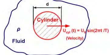
As a first step the paper considers the two-dimensional case of a rigid, smooth and circular cylinder undergoing transverse sinusoidal oscillations and immersed in a viscous fluid otherwise at rest, as illustrated by Fig. 1.

Figure 1. Scheme of the considered system. Then the incompressible Navier-Stokes problem can we formulated by eqn (1).

(

)

! !

" ! ! # $

%

= =

& '

+

( )

=

** + ,

--. /

(

+

0 0

&

=

cyl cyl

f f

sur T

t U

U u

dans u

p u

u t u

dans u

div

/ 2 sin .

0 ) (

0

1

µ

2

2

Introducing the characteristic physical quantities x=d×x*, t=T×t*, u=U0×u* and p= U0 2

× p* (where d is the cylinder diameter), eqn (1) can be rewritten in the following dimensionless form:

! " ! # $ % + & ' = & + ( ( = * * * . * * * 0 *) ( u R K p K u u K t u u div e c c c (2)

where t*, x*, u* and p* stand for dimensionless variables.

The dimensionless numbers appearing in eqn (2) are the Reynolds number Re and the Keulegan-Karpenter number Kc defined by eqn (3):

d

D

d

T

U

K

d

U

R

!

µ

"

2

and

=

=

=

where D is the maximal cylinder displacement.

So the physical system can be described by those two dimensionless numbers: Re compares the importance of the fluid viscosity to its inertia, and Kc measures the amplitude of the cylinder displacement compared to its diameter. We define the map (Kc ,Re) to study the variations of the in-line force acting on the cylinder Fcyl with time according to the configuration (Kc ,Re) of the physical system.

Various tools of analysis are used in that investigation. First we observe the evolution of the flow structure, notably the boundary layer and the vortices in the cylinder wake. They can be visualized by drawing for instance the velocity norm field, the pressure field or the vorticity field. Those figures allow us to analyse the curves of the cylinder force versus time. We also develop an interpretation of the force based on the global power balance eqn (4).

d c cyl cyl cyl P dt E d U F

P = . = + (4)

The cylinder power Pcyl is composed by an inertial power dEc/dt and a dissipative power Pd. The advantages and the relevance of that energy based method is that there is neither mathematical approximation nor limitation of validity in the map (Kc, Re). Moreover the decomposition has a precise physical meaning. It directly provides an expression of the exchanges between the fluid and the structure.

In particular we will measure the energy dissipated by the fluid thanks to the coefficient Qd defined by eqn (5) according to Duclercq (2008).Qd represents the normalized dissipative energy during an oscillation.

dt t U d dt t P Q cyl T T d d 3 0 0 ) ( 2 1 ) (

!

"

"

= (5)

3

NUMERICAL IMPLEMENTATION

Navier-Stokes equations and power balances are computed by means of a finite elements method. We solve the equations for the absolute velocity in the mobile reference frame linked to the cylinder in order to keep an invariant mesh. This is an Arbitrary Lagrangian-Eulerian (ALE) formulation without mesh deformation.

3

The equations of fluid motion are integrated using a two-dimensional DNS algorithm with a second-order finite-difference scheme for accurate prediction of the flow. Indeed a first-second-order temporal scheme generated artificial damping. The problem is then solved by projection and with a relaxation method to hasten convergence. For Kc≥1, the time step dt is chosen such as the CFL defined by CFL=Kc×dt /dx is equal to 0.05; for Kc≤1, the time step is equal to 0.05 cylinder oscillation period.

4

RESULTS

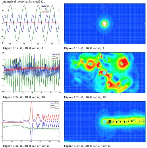
We consider the cases of Re=100, 500, 1000 then 2000 and Kc=0.125 to 50. For high values of Re and Kc, experiments have largely pointed out that the flow structure becomes three-dimensional and turbulent, as presented by Rajani (2008) for instance. However we carried out 2D-simulations for high Kc with the same numerical model as for small Kc.

Figure 2.1a.Re=1000 and Kc=1 Figure 2.1b.Re=1000 and Kc=1

Figure 2.2a.Re=1000 and Kc=10 Figure 2.2b.Re=1000 and Kc=10

Figure 2.3a.Re=1000 and infinite Kc Figure 2.3b.Re=1000 and infinite Kc

Figure 2. Left column (a): Evolution with time of the cylinder force (green), the inertial power (blue) and the dissipative power (red) for Re=1000 and different values of Kc.

4

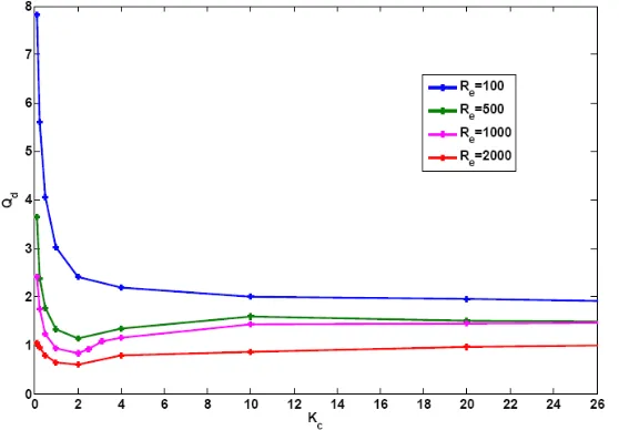
In this paper we would like to focus on the influence of the parameter Kc on the system behavior. That is why we present results for Re=1000 only. Regarding Kc, we select values representative of the main characteristic cases. Fig. 2 above presents the corresponding evolution versus time of the quantities from the energetic balance eqn (4) and a visualization of the flow structure. Then Fig. 3 gives the variations of the dissipative coefficient Qd defined by eqn (5) throughout the map (Kc, Re).

Figure 3. Dissipative coefficient Qd versus Kc for different values of Re.

Fig. 3 provides a characterization of the system behavior in terms of (Kc, Re). It appears different types of regimes that are studied in the following three sections.

4.1 Regime of very small Kc

The convective term in eqn (1) is negligible for low Kc and the Navier-Stokes equations are reduced to the linear Stokes (1851) equations. According to Cobbin (1995) and Sarpkaya (2001) the analytical solution for the force can be written as:

)

(

2

1

)

(

4

)

(

t

U

U

d

C

dt

t

dU

d

C

t

F

cyl m

cyl

=

!

"

+

!

where the inertial and drag coefficients, Cm and Cd, are defined from Bessel functions.

Stokes solution was later expanded by Wang (1968) to express Cm and Cd in terms of Kc and Re as Kc << 1 and Re /Kc >> 1. It leads to the following expression for Fcyl after having been reduced to its leading terms:

) ( 2 1 2 3 ) ( 4 ) ( 0 2 / 5 2 t U U d R K dt t dU d t F cyl e c cyl cyl

!

"

"

!

Then the analytical solution of Stokes and Wang injected in the general expression of Qd (eqn (5)) yields:

e c e c e c Stokes d R K R K R K

Q 26.24

2 3 ) , ( 2 / 5 =

=

!

That equation fits very well the numerical results of Qd (Kc) obtained on Fig. 3 for low Kc.

5

inertial power (Fig. 2.1a). Thus the cylinder force is proportional to its acceleration with a coefficient ma called the added mass since Fritz (1972). Indeed the fluid kinetic energy can be written as:

)

(

4

2

1

)

(

2

1

)

(

2 2

t

U

d

Q

t

U

m

t

E

=

=

"

!

where we defined the inertial coefficient Qc to measure the kinetic energy of the fluid. In the present example

Kc=1, Qc is equal to 1.74. It corresponds to the volume of fluid which is put in movement around the cylinder.

4.2 Asymptotic case: infinite Kc

As most hydrodynamic problems, it is of interest to explore the asymptotic behavior of the system. For very large values of Kc each cylinder half-oscillation can be regarded as the case of a cylinder in uniform translation in a fluid at rest, which is equivalent after changing the reference frame to the configuration of a uniform flow past a fixed cylinder. Many experimental and numerical investigations have given for the drag force the following semi-empirical formula eqn (10):

cyl cyl e

cyl t C_d R d U U

F

!

2 1 ) ( )

( = " (10)

That expression yields the asymptotic equation of Qd for infinite Kc:

)

(

2

3

)

(

K

d

R

C

R

Q

=

!

The asymptotic values on Fig. 3 indeed tend to the values of eqn (11) where Cd (Re) is given by the literature (see Chassaing (2005) for instance). We also directly implemented the resolution of the asymptotic problem and the results for Cd (Re) were in good agreement with the literature.

The computation of the kinetic energy in the present example Re=1000 gives Qc=23.6 (whereas Qcwas equal to 1.74 for Kc=1). Although the amount of kinetic energy looks high, the amplitude of its variations is equal to 1.0 only (whereas it was 1.6 for Kc=1). Consequently the dominant mechanisms for infinite Kc are dissipative effects. Note that the dimensions of the computational domain must have been taken into account for the analysis of Cd (Re) and Qc to fit with the data from literature (see Posdziech (2007) for instance).

In fact, for Re > 50 the flow presents vortex shedding. That structure, usually referred to as the Von Karman street, appears on Fig. 2.3b. The wake contains firstly contra-rotative vortices but then it is strongly disrupted by the right wall. The influence of the wall can also be observed on the fluctuations of the forces and the powers on Fig. 2.3a. The first variations of the curves at about t*=20 correspond to the destabilization of the wake: its symmetry is broken and the part of the wake at the extremity downstream breaks away; it is the onset of vortex shedding. Then a peak appears at t*=30, as the first vortex arrives on the exit wall and its energy is absorbed. From t*=43, a periodic regime takes place with a dimensionless vortex shedding frequency of 0.244 for Re=1000, which is in good agreement with the value of the Strouhal number versus Re given by Roushan (2005). Vortex shedding is the mechanism responsible for the dissipation characterizing the behavior of the system for infinite Kc.

4.3 Regime of transition: intermediate values of Kc

According to nuclear applications, attention is focused on intermediate values of Kc. In that region of the map (Kc ,Re), the Stokes and Wang’s solutions are not valid any more and the asymptotic regime is not yet reached. This regime of transition is characterized by an off-peak of the curves on Fig. 3 for high enough values of Re. A peak-off actually occurs if the value of Qd reached at the end of the range of validity of the Stokes equation is lower than its asymptotic value. More precisely, the value of Re from which an off-peak can be expected is determined by:

Re c

= min

{

|

(Kc, Re c

) < Qd Kc + ∞

(Re c

6 With the analytical expression of Qd

Stokes

(Kc, Re) (eqn (8)) given by Stokes and Wang (1968) and the data of Qd

Kc + ∞

(Re) (eqn (11)) given by Chassaing (2005), we find that Re c

is about equal to 500. The same critical value is obtained in the present computations on Fig. 3. For example the curve of Qd (Kc ,Re=1000) presents a minimum of 0.83 for Kc=2 whereas its asymptotic value is of 1.59.

The objective is now to understand the system’s behavior during the regime of transition for Re>Re c

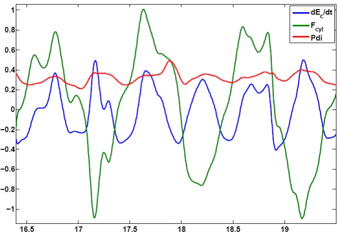
. The evolutions of the dissipative power, the inertial power and the cylinder force versus time are presented on Fig. 2.2a for Kc=10 and Re=1000. A zoom is also given on Fig. 4 below.

Figure 4. Evolution with time of the cylinder force (green), the inertial power (blue) and the dissipative power (red) for Re=1000 and Kc=10 (zoom of Fig. 2.2a).

Here the curves are not sinusoidal any more as for Kc=1. Moreover the dissipative power (in red) reaches the same order of magnitude as the inertial power (in blue), unlike the Stokes’ cases (Fig. 2.1a). The curves variations are also more complex than for infinite Kc (Fig. 2.3a).

The visualization of the vorticity field on Fig. 2.2b shows that the flow structure has been strongly disordered. In fact Kc is high enough to enable vortex shedding. Vortices collide with the vortices of the previous half-oscillation and with the cylinder on its way back. As a consequence the fluid contains much kinetic energy (Qc=97.1) fluctuating with a normalized amplitude of 2.1 (whereas the amplitude was 1.0 for infinite Kc).

Furthermore, in order to better understand how dissipative effects take place, we computed the local power balance for each element of the mesh. The aim is to see how the dissipation is distributed. Thus we calculated according to eqn (13) the quantity d of power dissipated in the elements placed before the abscissa Xfront for -L<Xfront<L (where L=10 cylinder diameters is the length of the fluid domain on both sides of the cylinder).

!

=

# Xfront

L d

d(t) P (x,t)dx for -L < Xfront < L (13)

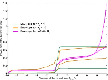
Thus Fig. 5 shows the envelopes of the variations of d (t) during a period as a function of Xfront for

7

Figure 5. Power d dissipated before the vertical front of abscissa Xfront, versus Xfront. The envelope of the fluctuations of d during a cylinder oscillation in periodic state is plotted for Re=1000 and Kc=1 (green), 10 (orange) and +∞ (pink). (The cylinder abscissa is Xcyl=0.)

For Kc=1 dissipation is localized around the cylinder and directly depends on the instantaneous cylinder velocity because the envelope of the fluctuations is very wide. For infinite Kc dissipation first takes place around the cylinder, but also in its wake (it increases linearly); nevertheless the presence of the right wall generates much dissipation, since it absorbs the vortices shed downstream of the cylinder. For Kc=10 dissipation is distributed on both sides of the cylinder. It can also be noticed that the envelope of the fluctuations is narrower than before. Indeed, even when the instantaneous cylinder velocity is zero, vortices are still present in the flow to maintain dissipative effects.

5

CONCLUSION

In this paper we presented the development of complementary tools to identify and characterize the different mechanisms governing the behavior of the system in terms of Kcand Re. Those tools are based on results of the numerical resolution of Navier-Stokes equations interpreted with physical considerations. Thanks to the visualization of the flow structure, the analysis of the variations of the force with time, and the determination of the global and the local power balances we measured the inertial and dissipative effects to understand the energetic exchanges between the cylinder and the fluid.

Then we focused on the case of Re=1000 to determine the influence of the parameter Kc on the cylinder force. For low Kcthe energy provided by the cylinder is mainly used by the fluid to induce its movement: the system has an inertial behavior. For very high Kc the flow is organized to dissipate the energy brought by the cylinder in vortices. For intermediate values of Kc both inertial and dissipative mechanisms are in competition. The variations of the cylinder force become irregular because of the disordered flow structure. The consequences of the collisions between the vortices and the cylinder on the force variations must be investigated more precisely. A noticeable feature of the regime of transition is also the minimum of the dissipative coefficient Qd.

8

REFERENCES

Broc, D., Duclercq, M. 2008. Toward a global model for FSI in tube bundles. Pressure Vessel and Piping paper PVP2008-61570.

Cobbin, A. M., Stansby, P. K. 1995. The hydrodynamic damping force on a cylinder in oscillatory, very-high-Reynolds-number flows. Applied Ocean Research. Vol. 17. P. 291-300.

Chassaing, P. 2005. Mécanique des fluides à l’usage de l’ingénieur. Institut pour la Promotion des Sciences de l’Ingénieur.

Duclercq, M., Broc, D. 2008. Physical and numerical study of the interaction between a fluid and an oscillating cylinder. Pressure Vessel and Piping paper PVP2008-61036.

Fritz, R. J. 1972. The Effect of Liquids on the Dynamic Motion of Immersed Solids. Journal of Engineering for Industry. Vol. 94. P. 167-173

Morison, J. R., O’Brien, M. P., Johnson, J. W., Schaaf, S. A. 1950. The forces exerted by surface waves on piles. Petroleum Transactions. AIME. Vol. 198. P. 149-157.

Posdziech, 0. ,Grundmann, R. 2007. A systematic approach to the numerical calculation of fundamental quantitites of the two-dimensional flow over a circular cylinder. Journal of Fluids and Structures. Vol. 23. P. 479-499.

Rajani, B. N., Kandasamy, A., Sekhar Majumdar 2008. Numerical simulation of laminar flow past a circular cylinder. Applied Mathematical Modelling.

Roushan, P., Wu, X. L. 2005. Structure-Based Interpretation of the Strouhal-Reynolds Number Relationship. Physical Review Letters. Vol. 94:5.

Sarpkaya, T. 2001. Hydrodynamic damping and quasi-coherent structures at large Stokes numbers. Journal of Fluids and Structures. Vol. 15. P. 909-928.

Schlichting, H. 2000. Boundary-Layer Theory. Springer. Sec. 4.8.

Stokes, G. G. 1851. On the effect of the internal friction of fluids on the motion of pendulums. Transactions of the Cambridge Philosophical Society. Vol. 9.