Difference -Analytical Method of The One-Dimensional
Convection-Diffusion Equation
Dalabaev Umurdin
Department mathematic modelling, University of World Economy and Diplomacy, Uzbekistan
Abstract. An analytical differencing scheme solution for the one-dimensional
convection-diffusion problems is presented. Deriving of an analytical solution is based on a differential equation difference analogue.
Key words: difference scheme,convection-diffusion, difference -analytical
Introduction
The method of finite differences [1] is most often used at a differential equation solution. The idea of a solution of boundary value problems is rather simple: instead of derivatives in a differential equation are used it finite difference approximations.
Convection-diffusion problems are base at modelling of problems of hydrodynamics and heat-mass transfer [2]. The basic attention at a numerical solution is given to problems of approximation of convective terms [2-6]. Upwind schemes, central differences, hybrid schemes, a high order upwind schemes are widely used. In the case of central differences, iterative methods for solving the resulting system of linear equations do not converge when the convective terms dominate. Schemes of a low order for the convection-diffusion equation connect unknown quantities in the three nodal points (UDS, CDS, Power law, hybrid schemes). For schemes of higher order nodes more than three will be required (QUICK, SMART, MINMOD, TOPUS etc.).
Usually, solution of differential equations by numerical methods is obtained in the form of numbers. Here we will show a possibility of deriving of a solution of differential equations by difference methods in the approximately-analytical form. This idea, which show’s for a one-dimensional convection-diffusion equation.
Difference-analytical method
Let's consider the one-dimensional convection-diffusion equation on a finite interval with boundary conditions:
2
2 ( )
e e
dФ d Ф
P P S x
dx = dx + ⋅ (1)
( ) W, ( ) E
Ф W =Ф Ф E =Ф (2)
where Pe V E W( ) Г
ρ −
= - Peclet number, ( )S x – a given
function, Ф unknown function.
We take an arbitrary point x∈[W E, ] and we will divide a segment on two parts (fig. 1). Flow direction is pointed fig. 1. We use upwind scheme. Then instead of (1) we have the difference -analytical equation
0 0 0 0 0 0
2
( )
W E W
e e
U U U U U U
P P S x
x W E W E x x W
− = − − − + ⋅
− − − − (3)
Here U0 value of unknown function in the nodal point x
(
UW0 ≡Ф UW, E0 ≡ФE)
. As [ , ]x∈ W E an arbitrary point from (3) we can define and receive the approached analytical solution of the problem (1)-(2):
(
)
(
)(
)
(
)(
)
0 0
0 2 2 ( ) ( )( )
( ).
2 ( ) 2 ( )
E e W
e
e e
x W U P E W E x U x W E x
U P S x
E W P E x P E x
− + + − − − −
= + ⋅
− + − + −
Let's note that, by this way of such approach some problems [7] are solved.
To improve approximate solution we take an additional nodes: 1 , 2 x W x = +
2 .
2 x E
x = + We will write the UDS scheme of type (3) for [ , ],W x [ ,x x1 2] and [ , ]x E . We will receive system from three equations. We exclude the received system, U x1( )1
and U x1( 2) as a result we will obtain the improved scheme:
(
)
(
)
(
)
1 1 1 1 1 1
1 1 1
4
( )
1 1 1
2 2 2
W E W
e e
U U U U U U
P P S x
x W τ E W E x γ x W τ
− − −
= − + ⋅ +
− + − − + − +
(
)
1 11 2
1 2
4 1 4 1
( ) ( )
1 1
e
P E W
S x S x
E W E W
τ γ
τ γ
+ ⋅ − − −
−
− + − + (4)
where 1 2 , 1 2 , ( ), ( ).
2 t 2 t P x We P Ee x
θ
τ = γ = + = − θ = −
+ In (3)
1
U is improved value
of unknown function in the nodal point x
(
UW1 ≡Ф UW, E1 ≡ФE)
.Solving (4) rather U1 we will receive the improved analytical solution. Again to improve solution we will arrive similarly: we will write the scheme (4) for [ , ],W x
fig. 1
W x E
1 2
[ ,x x ] and [ , ]x E , and we will exclude unknowns in points x1 and x2, etc. Continuing this process as a result we will have
1
2 2 2
2
( )
1 1 1
2 1 2 1 2 1
k k k
k k k k k k k
W E W
e
k k k
k k k
k k k
U U U U U U
P F x
E W
x W τ E x γ x W τ
τ γ τ + − = − − − + − − − − − − − − − − (5)
where 2 , 2 ,
2 2
k k
k k k k
t
θ
τ = γ = +
+
(
) (
)
21 2 1
1 2 1 1 1 2 ( ) ( ) 2 1 k k k j k i e
e k k
j i k
P E W x W
F x P S x S W j
E W τ τ τ + − − = = − + ⋅ − − = ⋅ + ⋅ + − − −
∑∑
(
)
2(
)
1 2 1
1 2 1 1 1 2 2 . 2 1 k k k j
k i k
k k
j i k
E x
S x j
E W γ γ γ + − − = = − ⋅ + − − − −
∑∑
In improved (5) Uk value of unknown function in a nodal point x
(
UWk ≡Ф UW, Ek ≡ФE)
. Solving the equation (5) rather Uk we will receive the approached analytical solution of an initial problem.If in (5) k =0 and summation to suppose equal to zero (an upper bound of the sum it is less than a limit inferior) then we will receive the scheme (3), at k =1 the scheme (4) etc. turns out.
Let's note that if from (5) we will define Uk and we will calculate that a lim k
k→∞U
gives an exact solution of corresponding problems.
Analytical examples
In order to verify the theory, the numerical computations were carried out with several S x( ).
On fig. 2 solutions of a problem (1) are reduced at R=20, S x( )=0 on [0;1] with boundary conditions ФW =0, ФE =1. On fig. 2 solutions of a problem (1) are reduced at R=50, S x( )=5cos 4x on [0;1] with boundary conditions
0, 1.
W E
Ф = Ф = From the graph it is visible that, in process of increase k to approximate solutions comes nearer to the exact.
From graphs it is visible that, since k =7 exact and approximate solution are visually coincides.
fig.2 fig.3
Continuous line – exact, point wise – k =0, dashed – k =1, point wise-dotted – 2
k = , long dashed – k =3, rare dashed – k =7
Numerical examples
The analytical scheme (5) allows not only receiving the approached analytical solution, but also gives the chance in creation of the qualitative scheme. For example, from (5) at in regular intervals disposition of nods of a grid with h we have the scheme:
1 1
2
k k k k
i i i i i i k i
h c U =bU+ +a U− + F
(6)
where
2 2
1 1 1
, , 1 , , ,
2 1 1 k 1 k
h k k
k k k k k i i k i i i
k k
k
P g e
R e g R b a g c a b
R g e
− −
= = = + = = = +
+ − − ,
(
)
(
)
(
)
2 2 1
1 1 2
1 1
2 2 1
1 2
1 1
1 2
( )
2 1
1 2
2 .
2 1
k
k
k
k
k j
k k n
i e i e k i k
j n k
k j
k n k
k i k
j n k
e h
F P S x P e S x j
h e
g h
g S x j
h g
−
− −
= =
−
−
= =
−
= ⋅ + + + −
−
−
+ −
−
∑∑
∑∑
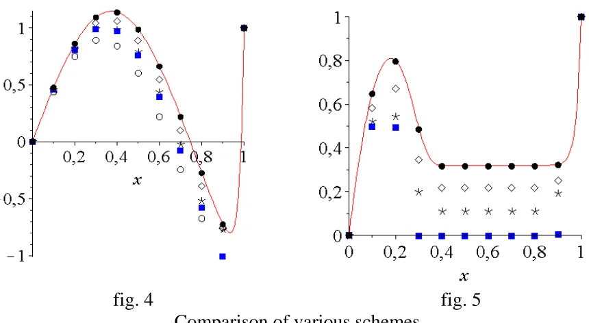
Here Ph =ρVh/Г so-called grid Peclet number, xi =W +ih nodal points. Comparisons of exact and difference solutions are on fig. 4 and 5 reduced.
fig. 4 fig. 5 Comparison of various schemes
Solution of problem (1) at Pe =50 are on fig. 3 and 4 graphs on [0;1] with boundary conditions ФW =0, ФE =1. Fig. 4 corresponds at ( )S x =5cos 4x and graphs on fig. 5 are received at
10 50 0,3
( ) 50 20 0,3 0, 4
0 0, 4 x if х
S x x if x
if x
− ≤
= − < <
<
Numerical results are received at h=0,1 and Ph =5. Solid lines of a drawing of exact solutions of a problem. Circle numerals are received for UDS scheme, rectangles under the scheme of Patankar, an asterisk on (6) at k =1, диамант at k =2 and circles at k =7. From fig. 4, 5 appears that, the offered schemes yield good results.
Conclusions
By an example of a one-dimensional problem the new set of analytical schemes is offered. By these schemes it is possible to receive an analytical solution. Testing of the offered schemes by example of stationary modelling boundary value problems is held.
Test calculations confirm efficiency of application of the difference -analytical scheme for solution convection-diffusion problems.
References
[1] Samarskii, A. A. The Theory of Difference Schemes. Monographs and
Textbooks in Pure and Applied Mathematics, 240. Marcel Dekker, Inc., New York, (2001).
[2] Patankar S.V. Numerical heat transfer and fluid flows. New York: Hemisphere Publishing Corporation; (1980).
[3] Leonard B.P. A stable and accurate convective modelling procedure based on quadratic upstream interpolation. Comput Methods Appl Mech Eng 19:59–98.
(1990)
[4] Leonard, B.P., S. Mokhtari, Beyond first-order upwinding: the ultra sharp alternative for non-oscillatory steady-state simulation of convection, Int. J. Numer. Methods Eng., 30, 729(1990)
[5] Leonard, B.P. The ULTIMATE conservative difference scheme applied to unsteady one-dimensional advection. Comp. methods applied mech. eng. 1991. Vol. 88. pp. 17-74.
[6] Ferreira V.G., de Queiroz R.A.B., Lima G.A.B., Cuenca R.G., Oishi C.M., Azevedo J.L.F., McKee S.. A bounded upwinding scheme for computing convection-dominated transport problems. Computers and Fluids 57(2012) pp. 208-224
[7] U.Dalabaev About one mode of average differential the equation and its application for a solution of problems of a mechanics of a liquid, Modern problems of a mechanics, lecture and theses, October, 29-31th 2001, Tashkent, pp. 113-118