The Numerical Solution of the Fredholm Integral Equations of the Second
Kind
Ali Aeed Mohammed
Master of Science (Applied Mathematics), Department of Mathematics University College of Science, Osmania University
ABSTRACT:
In this thesis we focus on the mathematical and numerical aspects of the Fredholm integral equation of the second kind due to their wide range of physical application such as heat conducting radiation, elasticity, potential theory and electrostatics. After the classification of these integral equations we will investigate some analytical and numerical methods for solving the Fredholm integral equation of the second kind. Such analytical methods include: the degenerate kernel methods, the Adomain decomposition method, the modified decomposition method and the method of successive approximations. The numerical methods that will be presented here are: Projection methods including collocation method and Galerkin method, Degenerate kernel approximation methods and Nystrom methods. The mathematical framework of these numerical methods together with their convergence properties will be analyzed. Some numerical examples implementing these numerical methods have been obtained for solving a Fredholm integral equation of the second kind. The numerical results show a closed agreement with the exact solution.
Keywords: Fredholm integral equation, Galerkin method, Nystrom methods
INTRODUCTION:
The subject of integral equations is one of the most important mathematical tools in both pure and applied mathematics. Integral equations play a very important role in modern science such as
numerous problems in engineering and mechanics, for more details. In fact, many physical problems are modeled in the form of Fredholm integral equations, such problems as potential theory and Dirichlet problems which discussed, electrostatics, mathematical problems of radiative equilibrium, the particle transport problems of astrophysics and reactor theory, and radiative heat transfer problems which
discussed,. Many initial and boundary value problems associated with ordinary differential equations (ODEs) and partial differential equations (PDEs) can be solved more effectively by integral equations methods. Integral equations also form one of the most useful tools in many branches of pure analysis, such as the theories of functional analysis and stochastic processes. Definition
An integral equation is an equation in which the unknown function to be determined appears under the integral sign. A standard integral equation is of the form
( ) ( ) ∫ ( ) ( ) ( ) ( )
(1.1)
Where ( ) and ( ) are limits of integration, is a constant parameter, and ( ) is a function of two variables and called the kernel of the integral equation. The function that will be determinedappears under the integral sign, and sometimes outside the integral sign.The functions ( ) and ( ) are known and ( ) is the unknown function. Thelimitsofintegration ( )and ( ) may be both variables, constantsor mixed, and they may be inone dimension or two or more.
Fredholm integral equations
The most standard form of Fredholm integral equations is given by the form
( ) ( ) ( )
∫ ( ) ( ) ( )
withD a closed bounded set in , for some m ≥ 1 .
Case(i)If the function ( ) ( )
yields
( )
P a g e | 1333 The equation involved the unknown function
only under the integral sign. In this case the integral equation is called Fredholm integral equation of the first kind.
Case( i i )If the function ( )
then(1.2)becomes
( ) ( ) ∫ ( ) ( ) (1.4) The equation involved the unknown function both inside as well as outside the integral equation. In this casetheequation is called Fredholm integral equation of the second kind.
Case(iii)If ( ) is neither then (1.2)
called Fredholm integral equation of the third kind
Volterra integral equations
The most standard form ofVolterra integral equations is given by the form
( ) ( ) ( ) ∫ ( ) ( ) (1.5)
where the upper limit of integration is a variable and the unknown function appears linearly or nonlinearly under the integral sign.
Case(i)If the function ( ) then equation
(1.5) becomes
( )
∫ ( ) ( )
(1.6)
The equation involved the unknown function appearsonly under the integral sign. In this case theintegral equation is called the Volterra integral equation of the first kind.
Case(ii) If the function ( ) then equation
(1.5) becomes
( ) ( )
∫ ( ) ( ) ( )
The equation involved the unknown function both inside as well as outside the integral sign. In this case the Integral Equation is called the volterra integral equation of the second kind.
Case(iii)If ( ) is nither nor then (1.5)
called Volterraintegral equation of the third kind. Singular integral equations
When one or both limits of integration become infinite or when the kernel becomes infinite at one or more points within the range of integration, the integral equation is called singular. For example,
( ) ( ) ∫ (
| |) ( ) ( )
is a singular integral equation of the second kind. Case (i)Singular Integral Equation: The kernel is of the form
( ) ( )
Where ( ) is a differentiable function of
( ) with ( ) then the integral equation is said to be a singular equation with Cauchy kernel where the integral
∫ ( )
( )
is understood in the sense of Cauchy Principal Value (CPV) and the notation P.V
∫ ( )
is usually used to denote this. Thus
∫ ( ) {∫ ( ) ∫ ( ) }
Case(ii)Weakly singular integral equation: Here the kernel is of the form
( ) ( ) | |
Or
( ) ( ) | |
Where ( ) is bounded
( ) ∫ ( ) ( )
(1.9)
Is a singular integral equation with a weakly singular kernel.
Case (iii) Strongly singular integral equations : If the kernel ( ) is of the form
( ) ( )
( )
Where ( ) is a differentiable function of
( )with ( ) , then the integral equation is said to be a strongly singular integral equation. For more details see [22].
Integro Differential equations
In this type of equations, the unknown function appears as a combination of both ordinary derivative and under the integral sign. In the electrical engineering problem, the current ( ) flowing in a closed circuit containingresistance, inductance and capacitance is governed by the following integro-differential equation,
∫ ( )
( ) ( )
Where L is the inductance, R the resistance, C the capacitance, and ( ) be the applied voltage. Similar examples can be cited as follows
( ) ∫ ( ) ( ) (1.11)
( ) ( )
∫ ( ) ( ) ( ) ( ) ( )
SOLVING FREDHOLM INTEGRAL
EQUATIONS OF THE SECOND KIND: The existence and uniqueness
Some integral equation has a solution and some other has no solution or that it has an infinite number of solutions, the following theorems state the existence and uniqueness among the solution of Fredholm integral equation of the second kind.
Note: It is important to say that we will discuss the analytical methods in the space
, -
Theorem (Fredholm alternative)
Either the nonhomogeneous linear equation of second kind
( ) ( ) ∫ ( ) ( ) ( )
has a unique solution for any function ( ) (in some sufficiently broad class) or the corresponding homogeneous equation
( ) ∫ ( ) (2.2)
has at least one nontrivial (that is, not identically zero) solution.
Theorem. If the first alternative holds true for equation (2.1), then it holds true for the associated equation
( ) ( ) ∫ ( ) ( ) (2.3)
as well. The homogeneous integral equation (2.2) and its associated equation
( ) ∫ ( ) ( ) (2.4)
P a g e | 1335
Note: If the functions ( ) ( ) ( )
are solutions of the homogeneous equation (2.2), then their linear combination
( )
( ) ( ) ( )
∑ ( ) ( )
where the ( ) are arbitrary constants, is also a solution of the equation.
Theorem. A necessary and sufficient condition for the existence of a solution ( ) of the non-homogeneous equation (2.1) in the latter case of the alternative is the condition of a orthogonality of the right side of the equation, i.e., of the function ( ), to any solution ( ) of the homogeneous equation (2.4) associated with (2.2)
∫ ( ) ( )
Some Analytical Methods for solving
Fredholm integral equations of the second kind
The degenerate kernel method
The kernel ( ) of a Fredholm integral equation of the second kind is called degenerate if it is the sum of a finite number of products of functions of alone by functions of alone, i.e.., if it is of the form
( )
∑ ( ) ( )
( )
We shall consider the functions
( ) ( ) ( ) continuous in the basic square and linearly independent. The integral equation with degenerate kernel (2.6).
( ) ( )
∫ [∑ ( ) ( )
] ( ) ( )
is solved in the following manner .
Rewrite (2.7) as,
( ) ( )
∑ ( ) ∫ ( ) ( )
( )
and introduce the notation
∫ ( ) ( ) ( )( )
Then (2.8) becomes
( ) ( ) ∑ ( )
(2.10)
Where are unknown constants, since the function ( ) is unknown. Thus, the solution of an integral equation with degenerate kernel reduces to finding the constants (
) Putting the expression (2.10) into the integral equation (2.7), we get
∑ * ∫ ( ), ( ) ∑ ( )- + ( )
Whence it follows, by virtue of the linear independence of the functions ( )(
) that
∫ ( ), ( ) ∑ ( )-
Or
For the sake of brevity, we introduce the notations
∫ ( ) ( )
∫ ( ) ( )
And find that
∑ ( )(2.11)
Or, in expanded form
( ) ( )
( ) | |
(2.12)
For finding the unknowns we have a linear system of n algebraic equation in n unknowns. The determinant of this system is
( )
| |
|
|
(2.13)
For all values of for which ( ) the algebraic system (2.11), and there by the integral equation (2.7), has a unique solution. On the other hand, for all values of for which ( ) becomes equal to zero, the algebraic system (2.11), and with it the integral equation (2.7), either is insoluble or has an infinite number of solutions. Note that we have considered only the integral equation of the second kind, where alone this method is applicable.
Example solve the integral equation
( ) ∫ ( ) ( ) (2.14)
Now, write the equation (2.14) in the following from,
( ) ∫ ( )
∫ ( )
∫ ( )
We introduce the notation
∫ ( )
∫ ( ) ∫ ( ) (2.15)
Where are unknown constants. Then equation (2.14) assumes the form
( )
(2.16)
Substituting expression (2.16) into (2.15), we get
∫ (
)
∫ (
)
∫ (
)
P a g e | 1337
( ∫
)
∫
∫
∫
∫
(
∫
)
∫
∫
∫ ∫ ( ∫ )
∫
By evaluating the integrals that enter into this system we obtain a system of algebraic equations for finding the unknowns
}
(2.17)
The determinant of this system is
( ) |
|
The system (2.17) has a unique solution
Substituting the values of thus found into (2.16) we obtain the solution of the given integral equation
( ) ( )
For more examples see [54]
The Method of successive approximations : Neumann’s series
The successive approximation method, which was successfully applied to Volterra integral equations of the second kind, can be applied even more easily to the basic Fredholm integral equations of the second kind:
( ) ( )
∫ ( ) ( ) ( )
We set ( ) ( ). Note that the zeroth approximation can be any selected real-valued function ( ), . Accordingly, the first approximation ( ) of the solution of
( ) is defined by
( ) ( )
∫ ( ) ( ) ( )
The second approximation ( ) of the solution
( ) can be obtained by replacing ( ) in equation (2.19) by the previously obtained
( ) hence we find
( ) ( ) ∫ ( ) ( ) (2.20)
( ) any selective real valued function
( )
( ) ∫ ( ) ( ) (2.21)
Even though we can select any real-valued function for the zeroth approximation ( ) the most commonly selected functions for ( ) are
( ) We have noticed that with the selection of ( ) the first approximation ( ) ( ). The final solution
( ) is obtained by
( ) ( )
(2.22)
So that the resulting ( ) is independent of the choice of ( ). This is known as Picard’s method.
The Neumann series is obtained if we set
( ) ( ) such that
( ) ( ) ∫ ( ) ( )
( ) ∫ ( ) ( )
( )
( ) ( 23)
Where
( )
∫ ( ) ( ) ( )
The second approximation ( ) can be obtained as
( ) ( ) ∫ ( ) ( )
( ) ∫ ( )* ( ) ( )+
( ) ( )
( )( )
Where
( )
∫ ( ) ( ) ( )
Proceeding in this manner , the final solution
( ) can be obtained
( ) ( ) ( ) ( ) ( )
( ) ∑ ( ) ( )
Where
( )
∫ ( ) ( ) ( )
Example
Solve the Fredholm Integral equation
( ) ∫ ( )
By using the successive approximation method.
For solution let us consider the zeroth approximation is ( ) and then the first approximation can be computed as
( )
P a g e | 1339
∫
Proceeding in this manner,we find
( )
∫ ( )
∫ ( )
. /
Similarly, the third approximation is
( )
∫ (
)
. /
Thus, we get
( ) {
}
And hence
( )
( )
∑
. /
This is the desired solution.
Numerical Methods for Solving Fredholm Integral Equations of the Second Kind
Degenerate kernel approximation methods
We discussed the degenerate kernel method as an analytical method in chapter two (2.3.1) for solving the Fredholm integral equation
( ) ( ) ∫ ( ) ( )
(3.1)
with and , for some , where D is a closed and bounded set.
We said that the kernel ( ) is degenerate if it can be expressed as the sum of a finitenumber of terms, each of which is the product of a function of only and a function of only such that
( )
∑ ( ) ( )
( )
but most kernel functions ( ) are not degenerate. So that in this chapter we seek to approximate them by degenerate kernels.
The solution of the integral equation by the degenerate kernel method
In the view of the integral equation (3.1), the kernel function ( ) is to be approximated by a sequence of degenerate kernel functions,
( ) ∑ ( ) ( )
(3.3)
(3.4)
Where the associated integral operator is defined as
( ) ∫ ( ) ( ) ( ) (3.5)
Where is a closed bounded set in for some
and using ( ) with such that
( ) ( ) is compact.
We can write the integral equation (3.1) in the operator from as
( ) (3.6)
Then (3.6) can be written using (3.5) as
( ) (3.7)
Where is the solution of the approximating equation. Using the formula (3.3) for ( ) the integral equation (3.7) becomes
( )
( ) ∑ ( ) ∫ ( ) ( ) (3.8)
And using the technique discussed in section
(2.31) we have
( ) ( ) ∑ ( ) (3.9)
Where
∑
(3.10)
Such that
∫ ( ) ( ) (3.11)
And
∫ ( ) ( ) (3.12)
Are known constants. Again as we stated in section (2.31) equation (3.10) represents a system of algebraic equations for the unknowns whose determinant ( ) is given by
( ) | |
| |
(3.13)
Which is a polynomial in of degree at most n,that is not identically zero.
To analyze the solution of (3.1) by the degenerate kernel method the following situations arise:
Situation I: when at least one right member of
the system (3.9) is non zero, the following two cases arise under this situation.
(i) If ( ) , then a unique non zero solution of system (3.10) exists and so (3.1) has unique non zero solution given by (3.9). (ii) If ( ) , then the system
(3.10) have either no solution or they possess infinite solution and hence (3.1) has neither no solution or infinite solution.
Situation II:When ( ) , then (3.11) shows
that for Hence the system (3.10) reduces to a system of homogeneous linear equation. The following two cases arises under this situation.
(i) If ( ) , then a unique non zero solution
of the system (3.10) exists and so we see that (3.1) has unique zero solution ( ) (ii) If ( ) , then the system
P a g e | 1341 non zero solutions, those value of
for which ( ) are known as eigenvalues and any nonzero solution of the homogeneous Fredholm integral equation
( ) ∫ ( ) ( ) is known as a corresponding eigenfunction of integral equation.
Situation III: When ( ) but
∫ ( ) ( ) ∫ ( ) ( ) ∫ ( ) ( ) (3.14)
that is ( ) is orthogonal to all the functions
( ) ( ) ( ) (3.15)
Then
are zeros and reduces (3.11) to a system of homogeneous linear equations. The following two cases arise under this situation
(i) If ( ) , then a unique zero solution
, and hence (3.1) has only unique solution ( ) . (ii) If ( ) , then the system
(3.10) possess infinite nonzero solutions and hence (3.1) has infinite nonzero solutions.
Taylor series approximation
Let ( ) is a continuous function of two variables and , then the Taylor series expansion of function at the neighborhood of any real number with respect to the variable is :
( ) ∑ ( ) ( ) (3.16)
and
( ) ∑ ( ) ( ) (3.17)
that mean the mth terms of Taylor expansion to the function at the neighborhood with respect to the variable .
Consider the one-dimensional integral equation
( ) ( ) ∫ ( ) ( ) (3.18)
Often we can write as a power series in ,
( ) ∑ ( )( ) (3.19) or in
( ) ∑ ( )( ) (3.20)
Let denote the partial sum of the first n terms on the right side of (3.19)
( ) ∑ ( )( )
(3.21)
Using the notation of (3.3), is a degenerate kernel with
( ) ( ) ( ) (3.22)
The linear system (3.14) becomes
∑ ∫ ( )
( )
∫ ( )( ) (3.23) and the solution is given by
( ) ( ) ∑ ( )(3.24)
The integrals in (3.23) must often be calculated numerically. However, there is not much that can be said for integrals of this generality. First, they involve the entire interval [a, b], as contrasted with some later methods we consider. In addition, most of the integrands will be zero or quite small, in the neighborhood of , the left end of the interval. The latter may aid in choosing a more efficient method of numerical integration. The following example avoids the numerical calculation of most of these integrals.
Interpolator degenerate kernel
approximations
Interpolation is a simple way to obtain degenerate kernel approximations. There are many kinds of interpolation, but we consider interpolation using only the values of
trigonometric polynomials, piecewise polynomial functions (including spline functions), and others. We give a general framework for all of these,
Let ( ) ( ) be a basis for the space of interpolation functions we are using. For example, with polynomial interpolation of degree , we would use
( )
(3.25)
Let be interpolation nodes in the integration region D. The interpolation problem
is as follows: Given data f i n d
( ) ∑ ( )(3.26) With
( )
(3.27)
Thus, we want to find the coefficients solving the linear system
∑ ( )
(3.28)
In order for the interpolation problem to have a unique solution for all possible data { }, it is necessary and sufficient that
( ) , ( )- (3.29)
With polynomial interpolation and the basis of (3.25)
[ ]
This is called a Vandermonde matrix, and it is known that ( ) for all
distinct choices of .
To give an explicit formula for ( )we introduce a special basis for the
interpolation method. Define ( )to be the interpolation function for which
( )
Then the solution to the interpolation problem is given by
( ) ∑ ( ) (3.30)
For polynomial interpolation, this is called Lagrange’s form of the interpolation polynomial.
We often use this name when dealing with other types of interpolation, and the functions ( ) are usually called Lagrange basis functions. With polynomial interpolation,
( ) ∏ ( )
Interpolation with respect to the variable t Define ( ) ∑ ⏟ ( ) ( ) ( ⏟ ) ( ) (3.31)
Then ( ) ( ) all . For the case D = [a, b],
With ( ) being considered on the domain
, - , -, we have that
( ) ( )alongall lines . The linear system associated with the degenerate kernel method ( ) is
∑ ∫ ( ) ( )
∫ ( ) ( ) (3.32) The solution, is given by,
( ) ( ) ∑ ( ) (3.33) Note the integrals in (3.32) must generally be evaluated numerically.
When analyzing this degenerate kernel method within the context of the space ( ), the error depends on
‖ ‖ ∫ | ( ) ( )|
(3.34)
which in turn depends on the interpolation error ( ) ( ). Some special cases are considered below.
NUMERICAL EXAMPLES AND RESULTS
In this chapter we try to apply some of the numerical methods illustrated in chapter three to approximate the solution of the Fredholm integral equation
( ) ( ) ∫ ( ) ( ) (4.1)
These methods include: the degen erate
kern el meth od, the Nystr ̈m
methodandth e collocation method we
P a g e | 1343 then we will compare the exact solution with the
approximate one using suitable number of n points.
The numerical realization of equation (4.1) using the degenerate kernel method
First we expand the kernel ( )withrespect to t using the Taylor seriessuch that
( ) ∑ ( ) ( ) (4.2)
where m is the number of Taylor series terms, by this expansion, the kernel can be written as the sum of two separated functions one with respect to , and the other with respect to , such that
( ) ∑ ( ) ( )
(4.3)
Where
( ) . /
( ) (4.4)
And
( ) ( ) (4.5)
then we calculate the values , and such that
∫ ( ) ( )
∫ ( ) ( ) (4.6)
using the relations in section 2.3.1, and the above relations, we have
∑ (4.7)
now putting this relations in the matrix form we have, where
, -
Where
such that I is the identity matrix,
[ ] , -
And the matrix
, -
The solution is given by
( ) ( ) ∑ ( ) (4.8)
The following algorithm implements the
degenerate k ernel meth od using the
Matlabsoftware.
Algorithm 1
1. Input a, b, ( ) ( )
2. Input the number of Taylor series terms m
3. Calculate the Taylor expansion of ( ) with respect to
from find ( ) ( ), 4. Calculate ∫ ( ) ( )
5. Calculate ∫ ( ) ( )
6. Calculate the matrix
| | | |
7. Calculate the determinate D(A) of matrix A 8. If ( ) go to step 12.
9. If ( ) the system has infinite number of solutions ,go to step 16
10. The system has unique solution
go to step 16 11. If go to step 15
12. If D(A) = 0, the system has infinite number of solutions, go to step 16, thesystem has unique solution 13. If ( ) the system has no real solution,
go to step 16
14. The solution of system is, - , - , -then
( ) ( ) ∑
( )
1. End.
For more details see [20].
By returning to3.1.2 and using algorithm 1, the kernel of this integral equation ( )
( )can be expanded using Taylor series for 5 terms as
( ) ( ) ( ) ( ) ( ) ( ) ( ) ( )
( ) ( ) }
(4.11) and
( ) ( ) ( ) ( ) ( ) }
(4.12)
The related Matlab program gives the following results.
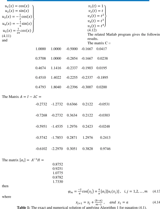
The matrix C =
1.0000 1.0000 -0.5000 -0.1667 0.0417
0.5708 1.0000 -0.2854 -0.1667 0.0238
0.4674 1.1416 -0.2337 -0.1903 0.0195
0.4510 1.4022 -0.2255 -0.2337 -0.1895
0.4793 1.8040 -0.2396 -0.3007 0.0200
The Matrix
-0.2732 -1.2732 0.6366 0.2122 -0.0531
-0.7268 -0.2732 0.3634 0.2122 -0.0303
-0.5951 -1.4535 1.2976 0.2423 -0.0248
-0.5742 -1.7853 0.2871 1.2976 0.2413
-0.6102 -2.2970 0.3051 0.3828 0.9746
The matrix , -
0.8752 0.9251 1.0775 0.8782 1.7330 then
( ) , -, ( )- (4.13) where
( ) (4.14)
P a g e | 1345 Analytical solution
( )
Approximate solution
Error = | |
0 0 -0.116299822082018 0.116299822082018
0.3927 0.382683432365090 0.271988984127792 0.110694448237297
0.7854 0.707106781186547 0.618869933090427 0.088236848096121
1.1781 0.923879532511287 0.871533544809957 0.052345987701329
1.5708 1.000000000000000 0.991514074803429 0.008485925196571
Figure 2: shows the exact solution ( ) ( ) and the approximate one when
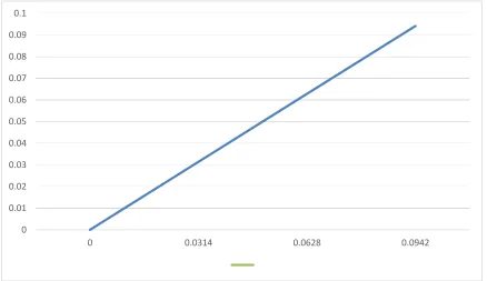
The exact and numerical solution of applying Algorithm 1 for equation (4.1). While Figure shows the absolute error which approaches zero.
0 0.2 0.4 0.6 0.8 1 1.2
0 0.2 0.4 0.6 0.8 1 1.2 1.4 1.6 1.8
Y-ax
is
Figure 3: The resulting error of applying algorithm 1 to equation (4.1).
The numerical realization of equation (4.1)
using the Nystr ̈m method
To solve the Fredholm integral equation of the second kind which is given by
( ) ( ) ∫ ( ) ( )
byNystr ̈m method, first we should remember that the kernel ( ) and the function
( ) must be continuous, secondly, we should know that we can approximate the
integral ∫ ( ) using quadrature rule by
∑ ( ). By such approximation, for
, the Fredholm integral equation
( ) ( ) ∫ ( ) ( ) (4.15)
can be reduced to
( ) ∑ ( ) ( ) ( ) (4.16)
where its solution ( ) is an approximation of the exact solution ( ) to (4.15). A solution to a
functional equation (4.16) can be obtained if we assign to in which and
. In this way, (4.16) is reduced to a system of equations
( ) ∑ ( ) ( ) ( ) (4.17)
Next, writing the equation (4.17) in the matrix form
( ) (4.18)
where
, ( )- , ( )- [ ( )]
( )
It's worth to mention that in order to approximate the integral, we will use the Trapezoidal Rule.
Here, we implement it in the form such that 0
0.02 0.04 0.06 0.08 0.1 0.12 0.14
P a g e | 1347
∫ ( ) ∑ (
)
(4.19)
where D is a diagonal matrix such that the elements of its diagonal equal h where h depends on the initial and the end points of the interval [a, b], and the number of the approximations n such that .The elements of the matrix
consist of the entries ( ) where
such that the approximations
obtained as , where
and
The following algorithm implements the
Nystr ̈m methodusing the Matlabsoftware.
Algorithm 2
Input ( ) ( )
For
End
For
( )
is diagonal matrix
For
( )
end
identity matrix
the answer of
( ) the interpolating polynomial at ,
-Table shows the exact solution ( )
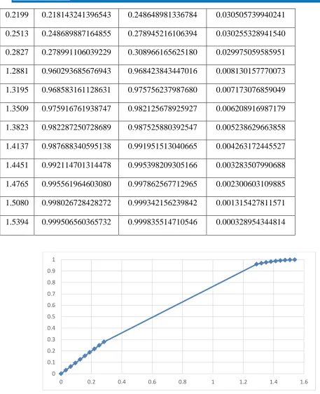
( ) and the approximate one when , and showing the error resulting of using the numerical solution.
Note: The table shows the first 10 values and the last 10 values only
Table The exact and numerical solution of
applying Algorithm for equation ( )
x
Analytical solution
( )
Approximate solution
Error | |
0 0 0.031405592470328 0.031405592470328
0.0314 0.031410759078128 0.062780191412531 0.031369432334402
0.0628 0.062790519529313 0.094092833885359 0.031302314356046
0.0942 0.094108313318514 0.125312618091103 0.031204304772588
0.1257 0.125333233564304 0.156408733871965 0.031075500307661
0.1571 0.156434465040231 0.187350493115954 0.030916028075723
0.2199 0.218143241396543 0.248648981336784 0.030505739940241
0.2513 0.248689887164855 0.278945216106394 0.030255328941540
0.2827 0.278991106039229 0.308966165625180 0.029975059585951
1.2881 0.960293685676943 0.968423843447016 0.008130157770073
1.3195 0.968583161128631 0.975756237987680 0.007173076859049
1.3509 0.975916761938747 0.982125678925927 0.006208916987179
1.3823 0.982287250728689 0.987525880392547 0.005238629663858
1.4137 0.987688340595138 0.991951513040665 0.004263172445527
1.4451 0.992114701314478 0.995398209305166 0.003283507990688
1.4765 0.995561964603080 0.997862567712965 0.002300603109885
1.5080 0.998026728428272 0.999342156239842 0.001315427811571
1.5394 0.999506560365732 0.999835514710546 0.000328954344814
Figure 4: The exact and numerical solution of applying Algorithm 2 for equation ( )
The CPU time is 0.064010 seconds.
The error analysis of the Nystr ̈m method
If we consider the trapezoidal numerical integration rule
0 0.1 0.2 0.3 0.4 0.5 0.6 0.7 0.8 0.9 1
P a g e | 1349
∫ ( ) ∑ ( ) (4.20)
with and for . The notation means the first and last terms are to be halved before summing. For the error,
∫ ( ) ∑ ( ) ( ) ( )
, - (4.21)
with some point in , - There is also the asymptotic error formula
∫ ( ) ∑ ( ) , ( ) ( )- ( ) , - (4.22)
When this is applied to the integral equation
( ) ( ) ∫ ( ) ( )
(4.23)
we obtain the approximating linear system
( ) ( ) ∑ ( ) ( )
(4.24)
which is of order
The Nystrom interpolation formula is given by
( ) ( ) ∑ ( ) ( ) (4.25)
The speed of convergence is based on the numerical integration error
( ) ( ) ( ) 0 ( ) ( ) 1 (4.26)
with ( ) , -. From ( ), the asymptotic integration error is
( ) ( ) 0 ( ) ( ) 1 ( ) (4.27)
From ( ), we see the Nystr ̈m method converges with an order of ( ), provided
( ) ( ) is twice continuously differentiable with respect to , uniformly in For more details see , -.
These results show that the algorithm , yields acceptable results since the maximum absolute error which is ( )
The numerical realization of equation (4.1) using the Collocation method
First we expand the function ( ) as a sum of basis * + such that
( ) ∑ ( ) 0 1 (4.28)
Since the residual ( ) can be written as
( ) ( ) ∫ ( ) ( ) ( ) (4.29)
Then by substituting (4.15) into the equation (4.16) so as to determine the values of the coefficients * + such that
( ) ∑ { ( ) ∫ ( ) ( ) } ( ) (4.30)
But we pick distinct node points such that
( ) (4.31)
Then ( ) can be rewritten as
∑ { ( ) ∫ ( ) ( ) } ( ) (4.32)
In this example we have , - (
We introduce the language basis functions for piecewise linear interpolation as
( ) { | |
(4.33)
Where the subspace is the set of all functions that are piecewise linear on [a,b], with
breakpoints * +. Its dimension is .
The projection operator is defined by
( ) ∑ ( ) ( ) (4.34)
Now for convergence of ( )
{ ( ) , -
, -
(4.35)
Where the function is defined by
( )
| | | ( ) ( )|
(4.36)
And it is called the modulus of the function .This shows that for all
, - Now for any compact operator
, - , - Lemma (3.6) implies
‖ ‖ as .Therefore the results of Theorem (3.4) can be applied directly to the numerical solution of the integral equation
( ) For sufficiently large n, say
, the equation ( ) has a unique solution for each , - ; and we can write
‖ ‖ | | ‖ ‖
For ,
-‖ ‖ | | ‖ ‖ (4.37)
The linear system (4.32) takes the simpler form
( ) ∑ ( )∫ ( ) ( ) ( ) (4.38)
And we simplify the integral for
∫ ( ) ( ) ∫ ( )(
) ∫ ( )( ) (4.39)
We have calculated the integrals above
numerically using quadrature rules specifically Trapezoidal Rule which is of the form
∫ ( ) 0 ( ) ∑ ( )
( )1 (4.40)
Now substituting (4.39) in (4.38) and putting this relation in the matrix form we have
( ) (
( )) (4.41)
Where
, ( )-
, ( )- [ ( )] ( )
[ ] ,
-The following algorithm implements the collocation method using the Matlab Software.
Algorithm 3
Input ( ) ( )
For
P a g e | 1351 For
( )
is a diagonal matrix
For
( )
end
identity matrix
For
For
( )
( )
,
-Table 4.2 compare the exact solution ( )
( ) with the approximate one when
and showing the error resulting of using the numerical solution.
Table 3: The exact and numerical solution of applying Algorithm 3 for equation (4.1).
Analytical solution
( )
Approximate solution
Error = | |
0 0 -0.031467686762045 0.031467686762045
0.0314 0.031410759078128 -0.000000000000004 0.031410759078132
0.0628 0.062790519529313 0.031467686762042 0.031322832767271
0.0942 0.094108313318514 0.062904318716399 0.031203994602115
0.1257 0.125333233564304 0.094278871702702 0.031054361861602
0.1571 0.156434465040231 0.125560382825064 0.030874082215167
0.1885 0.187381314585725 0.156717981008673 0.030663333577051
0.2199 0.218143241396543 0.187720917465807 0.030422323930735
0.2513 0.248689887164855 0.218538596041232 0.030151291123623
0.2827 0.278991106039229 0.249140603406845 0.029850502632384
1.3195 0.968583161128631 0.962034086005045 0.006549075123586
1.3509 0.975916761938747 0.970338584991732 0.005578176947016
1.3823 0.982287250728689 0.977685476945429 0.004601773783260
1.4137 0.987688340595138 0.984067511370779 0.003620829224359
1.4451 0.992114701314478 0.989478389970310 0.002636311344168
1.4765 0.995561964603080 0.993912772860129 0.001649191742951
1.5080 0.998026728428272 0.997366283839667 0.000660444588605
1.5394 0.999506560365732 0.999835514710550 0.000328954344819
1.5708 1.000000000000000 1.001318028640015 0.001318028640015
Figure 4: shows the exact solution ( ) ( ) with the approximate one when ,
Figure 4: The exact and numerical solution of applying Algorithm 3 for equation (4.1).
The CPU time is 0.066202 seconds.
These results show that the algorithm yields acceptable results since the maximum absolute error which is 0.03 is less than or equal ( ).
Conclusion:
In this thesis we have presented some
analytical and numerical methods for solving a
fredholm integral equation of the second kind. 0
0.01 0.02 0.03 0.04 0.05 0.06 0.07 0.08 0.09 0.1
P a g e | 1353 The analytical methods are the degenerate kernel
methods,the Adomain decomposition method,
the modified decomposition method and the
method of successive approximations. Moreover,
we have used the following numerical methods:
Projection methods including collocation method
and Galerkin method, Degenerate kernel
approximation methods and Nystr ̈m methods,
for approximating the solution of the Fredholm
integral equations. The have presented each
numerical method as algorithm and applied these
algorithms on the same Freedholm integral
equation using Matlab Software; we have found
that the numerical solution was approximately as
the exact solution. The absolute error has
approached zero which was shown that
numerical results were acceptable.
Reference:
1. G. Adomian, Solving Frontier Problems
of Physics, TheDecomposition Method,
Kluwer, Boston, (1994).
2. R. Anderson, The Application and
Numerical Solution of Integral
Equations, Sijthoff and Noordhoff
International Published B. V., (1980).
3. D. Arnold, W. Wendland, On the
Asymptotic Convergence of Collocation
Methods,Mathematics of Computation,
vol.41, Issue 164, 349-381, (Oct., 1983).
4. K. Atkinson, The Numerical Solution of
Integral Equations of the Second Kind,
The press Syndicate of the University of
Cambridge, United Kingdom, (1997).
5. K. Atkinson, A Personal Perspective on
the History of the Numerical Analysis of
Fredholm Integral Equations of the
Second Kind, The University of Iowa,
July 25, (2008).
6. K. Atkinson and W. Han, Theoretical
Numerical Analysis: A Functional
Analysis Framework, 2nd edition,
Springer-Verlag, New York, (2005).
7. K. Atkinson and L. Shampine, Algorithm
876: Solving Fredholm Integral
Equations of the Second kind in
Matlab,ACM Trans. Math.Software, 34
(2008).
8. Z. Avazzadeh, M. Heydari and G.
Loghmani,A Comparison Between
Solving Two Dimensional Integral
Equations by the Traditional Collocation
Method and Radial Basis Functions,
Applied Mathematical Sciences, Vol. 5,
No. 23, 1145 -1152, (2011).
9. E. Babolian and A. Hajikandi, The
Approximate Solution of a Class of
Fredholm Integral Equations with a
Weakly Singular Kernel,Journal of
Computational and Applied Mathematics
10. C. Baker, The Numerical Treatment of
Integral Equations, Oxford Univ. Press,
(1977).
11. M. Bonis and C. Laurita, Numerical
Treatment of Second Kind Fredholm
integral equations systems on bounded
intervals, Journal of Computationaland
Applied Mathematics 217, 64 - 87,
(2008).
12. F. Bulbul and M. Islam, Investigation of
the Solution of a Fredholm Integral
Equation of First Kind with
un-symmetric Kernel by Using Fourier
Series,International Journal of Science
and Technology, Vol. 1 No.5, November