Practical Aspects of a Data-Driven Motion
Correction Approach for Brain SPECT
Andre Z. Kyme*, Brian F. Hutton, Senior Member, IEEE, Rochelle L. Hatton, David W. Skerrett, and
Leighton R. Barnden
Abstract—Patient motion can cause image artifacts in single photon emission computed tomography despite restraining measures. Data-driven detection and correction of motion can be achieved by comparison of acquired data with the forward projections. This enables the brain locations to be estimated and data to be correctly incorporated in a three-dimensional (3-D) reconstruction algorithm. Digital and physical phantom experiments were performed to explore practical aspects of this approach. Methods: Noisy simulation data modeling multiple 3-D patient head movements were constructed by projecting the digital Hoffman brain phantom at various orientations. Hoffman physical phantom data incorporating deliberate movements were also gathered. Motion correction was applied to these data using various regimes to determine the importance of attenuation and successive iterations. Studies were assessed visually for artifact reduction, and analyzed quantitatively via a mean registration error (MRE) and mean square difference measure (MSD). Re-sults: Artifacts and distortion in the motion corrupted data were reduced to a large extent by application of this algorithm. MRE values were mostly well within 1 pixel (4.4 mm) for the simu-lated data. Significant MSD improvements( 2) were common. Inclusion of attenuation was unnecessary to accurately estimate motion, doubling the efficiency and simplifying implementation. Moreover, most motion-related errors were removed using a single iteration. The improvement for the physical phantom data was smaller, though this may be due to object symmetry. Conclusion: These results provide the basis of an implementation protocol for clinical validation of the technique.
Index Terms—Image registration, motion compensation, single photon emission computed tomography (SPECT), three-dimen-sional (3-D) reconstruction.
I. INTRODUCTION
S
INGLE-photon emission computed tomography (SPECT) is a valuable diagnostic tool in functional imaging, how-ever, it is well recognized that patient motion during data acqui-sition can result in artifacts in the reconstructed image that may compromise accurate diagnosis [1]–[3]. Moreover, use of head restraint does not necessarily rectify the problem [4].Manuscript received June 26, 2002; revised January 9, 2003. This work was presented in part at the Australian and New Zealand Society of Nuclear Medicine Annual Scientific Conference, 2002. Asterisk indicates
corre-sponding author.
*A. Z. Kyme is with the Diagnostic Physics Group, Department of Nuclear Medicine and Ultrasound, Westmead Hospital, Sydney, NSW 2145, Australia (e-mail: [email protected]).
B. F. Hutton, R. L. Hatton, and D. W. Skerrett are with the Diagnostic Physics Group, Department of Nuclear Medicine and Ultrasound, Westmead Hospital, Sydney, NSW 2145, Australia.
L. R. Barnden is with the Department of Nuclear Medicine, Queen Elizabeth Hospital, Woodville, Adelaide 5011, Australia.
Digital Object Identifier 10.1109/TMI.2003.814790
Numerous motion correction methods have been described in the literature. Manual shifting of projections using visual align-ment [5] and fiducial marker alignalign-ment [6] has been used to correct in-plane motion and axial translation. The method of “temporal image fractionation” was used [7] to compile a set of motion-free data from multiple acquisitions by excluding motion-affected data. Cross correlation of multiple projection sets [8], [9] has also been used to exclude motion-affected data prior to reconstruction. Various electromagnetic and optical de-vices have been applied in SPECT and positron emission tomog-raphy (PET) to measure patient motion [10]–[12]. Fulton et al. used these data to correct fully general movements in SPECT using a three-dimensional (3-D), iterative reconstruction algo-rithm [12]–[14]. A different approach to motion correction uses forward projection of the SPECT reconstruction [15], [16] to determine the movements necessary for obtaining a consistent projection set, but these groups have restricted their investiga-tion to axial and transaxial translainvestiga-tions.
This work describes practical aspects in validating a novel, fully 3-D, data-driven motion correction method.
II. METHODS
A. General Methodology
The principles underlying our novel approach to 3-D motion correction and the feasibility of implementation are described briefly in previous work by this group [17], [18]. A more com-plete description is provided here.
We wish to estimate radionuclide distribution where denotes position in the 3-D-object space. We define the acquired projections in projection space according to
(1)
where is the th simultaneously-acquired group of
projec-tions, is the set and is given by
(2)
Let be the operation of forward projecting at the angles corresponding to the th group. We also define the process
(3)
where is the updated reconstruction obtained when an it-erative reconstruction algorithm reconstructs an arbitrary set of projections using an initial image estimate .
1) Identification of Misaligned Projections: Obtain the first estimate by reconstructing the full set of acquired projections
, with a flat (gray) image as the starting reconstruction
(4)
The subscript denotes that this reconstruction is uncorrected and, therefore, may contain motion artifacts. (The position vari-ables and have been left out for simplicity.)
To identify groups of projections corresponding to discrete locations of the brain, we compute the square of the norm of the difference between forward projections and acquired pro-jections. The similarity measure for two discrete (projection or object) functions and is given by
(5)
where is the number of nonzero elements in .
By calculating for each value of , sets of
can be identified for which the position/orientation of the brain was fixed, i.e., we identify such that
(6)
Here, is a subset of containing the indices of all acquired groups that were collected with the brain at, or “close” to, location .
2) Estimation of Motion: To estimate motion parameters for each change in brain location, consider using a transformation operator to apply a rigid-body transformation (three rotations, three translations) in the object space. The aim is to choose the
transformation so as to minimize , where here
is given by
(7)
i.e., is the set of forward projections generated from (the transformed) at all angles identified as belonging to
move-ment .
Denoting the optimized transformation from location
to location as , the set of ’s are sought using
a direct-search optimization algorithm.
3) Motion Correction: Form the partial reconstruction using projections acquired at the brain location
(8)
The superscript on indicates we take this to be the initial motion-corrected estimate.
If we define a cumulative transformation operator according to
(9)
then updated motion-corrected estimates are given by the recurrence relation
(10)
When , the motion-corrected result is
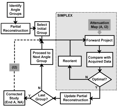
ob-tained. This can be returned to the initial frame of reference by applying the inverse cumulative transformation . Fig. 1 il-lustrates the general methodology.
Fig. 1. Flowchart describing the general methodology of data-driven motion correction and the different modes of correction. An attenuation map is used in the optimization cycle for modes A and I2 to account for attenuation (reconstruction and reprojection). Mode I2 involves a repeat of the cycle using the Mode A motion-corrected result as the starting reconstruction.
B. Implementation
1) Camera Geometry: This methodology is applicable for any multihead gamma camera geometry. We simulated dual-head 90 acquisition data for the digital phantom and ob-tained triple-head (120 ) acquisitions of the physical phantom. 2) Reconstruction: The operator was defined above as any iterative, tomographic reconstruction algorithm capable of updating some specified start image with an arbitrary set of pro-jections. We chose the ordered-subsets expectation-maximiza-tion (OSEM) algorithm [19]. The projecexpectation-maximiza-tion sets used in each motion-correction update were divided into OSEM sub-sets. For the digital phantom experiments, a subset size of two was used when of the data or less were available, otherwise a subset size of four was used. For the physical phantom experi-ments, projections were grouped together using a subset size of three.
3) Optimization: The similarity measure was mini-mized using the downhill simplex algorithm (maximum 250 function evaluations). Simplex was chosen for simplicity of implementation, its common use in registration problems, and its good performance in reasonably well-behaved parameter spaces.
Fig. 2. Similarity (MSD) between acquired and forward-projected data for the indexed angle pairs(p ) of a simulated phantom study. With no transformation of the reconstruction (a) was obtained. Transforming the reconstruction three different ways before calculating the similarity gave (b), (c), and (d). Note that at certain orientations of the brain [e.g., (b)] some movements may not be detected. These data suggest three distinct angle groups,P ; P ; P .
more conclusive picture of the motion relationships between an-gles, as can be seen in Fig. 2 for a dataset containing three head positions.
At present, identification of the motion groups from the mul-tiple versus curves is done visually. In future development, an automatic method will be investigated relying on the fact that variation of within a motion group tends to be much smaller than between groups (Fig. 2).
5) Partial Reconstruction: Instead of transforming (un-corrected reconstruction) to estimate the motion parameters for each movement (as per Section II-A), a partial reconstruction can be used. The partial reconstruction contains a consistent, but incomplete, set of projection data. First, we form the initial motion-corrected estimate as in (8), but choose as the largest of the ’s. Then, the ’s are obtained by minimizing the
similarity function , where in this case is given
by
(11)
i.e., is the set of forward projections generated from the th estimate at all angles identified as belonging to move-ment . Here, and updates proceed as before.
6) OSEM Subset Considerations: It has been suggested that OSEM reconstructions preferably should use subsets of well-dispersed angles in order to maximize information per sub-iteration [19]. This principle was applied to all OSEM reconstructions performed. Also, where possible, were chosen so that consecutive ’s did not correspond to spatially adjacent angle groups. In this way, progressive updates of the reconstruction had a more balanced addition of the available projection data.
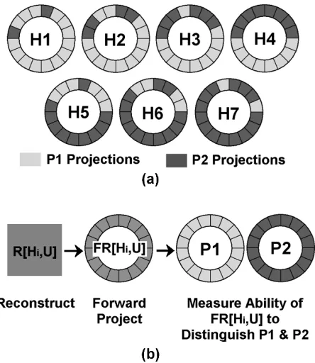
Fig. 3. (a) “Hybrid” projection sets formed by increasing the proportion of
P 2 projections. (b) Demonstrates how the “full” reconstruction was used to
determine how well data fromP 1 and P 2 could be distinguished. The hybrid set was reconstructed, forward projected, and the forward projections used to distinguish betweenP 1 and P 2. For the partial reconstruction, only projections inH that belonged to P 1 were used to reconstruct.
C. Basis for Using a Partial Reconstruction
The justification for using a partial reconstruction to get im-proved motion parameter estimates was obtained via the fol-lowing experiment: two complete projection sets and were generated by analytically projecting the digital Hoffman phantom at two different orientations. “Hybrid” projection sets were formed containing an increasing proportion of pro-jections [Fig. 3(a)]. To determine whether forward propro-jections generated from the fully or partially reconstructed data provided better differentiation between and , a distinguishability index was calculated as
(12)
where for full reconstruction and for partial recon-struction was the subset of belonging to . The oper-ator , without subscript, denotes forward projection at all an-gles. Fig. 3(b) illustrates the experiment.
Fig. 4 shows a plot of versus the number of projections contained in the full and partial reconstructions. For full recon-struction, the ability of the forward projections to differentiate and data rapidly declined to a minimum as the propor-tion of data in increased to 50%. By comparison, forward projections generated from the partial reconstruction showed an excellent ability to differentiate, even when of the data were used to reconstruct.
Fig. 4. Performance of forward projections generated from the full and partial reconstructions in distinguishing between the setsP 1 and P 2 (Fig. 3). Error bars represent the standard deviation of the MSD/projection values used to obtain the distinguishability index.
D. Data
1) Digital Phantom: Starting projection data for the simulations performed in this work were obtained by pro-jecting a 128 128 80 pixel (2.2-mm/pixel) version of the digital Hoffman brain phantom to 64 (64 40) projections (4.4-mm/pixel) using a high resolution, parallel-hole collimator model with attenuation but no scatter. Each pixel was replaced by a random, Poisson-distributed count after scaling the maximum counts/projection to 50 000.
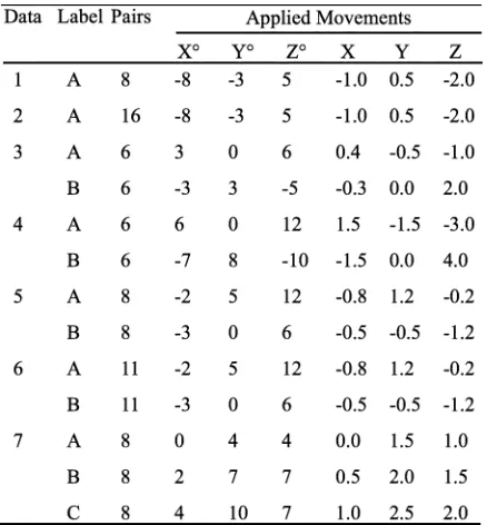
Projection data simulating an acquisition with head move-ment were generated by applying rigid-body transformations to the phantom, forward projecting, then combining projections from the resulting datasets. Seven studies simulating up to three head movements (four discrete positions) were created. The mo-tions included 3-D head tilting, twisting, and sliding—feasible movements resulting from coughing, discomfort, and tiredness of the patient in a clinical setting [4], [12], [20]. In addition, simulated sets varied in the angular location and extent of move-ment, and the magnitude in each degree of freedom (DOF). A summary of the motion-corrupted datasets is shown in Fig. 5 and Table I.
2) Physical Phantom: The Hoffman physical phantom data were acquired at a separate institution on a Philips Irix triple-head gamma camera ( MBq Tc, 120 projections (40/head), 30 s/proj., 3.5-mm/pixel). Three studies were col-lected: two had a single 3-D movement manually applied to the phantom for of the acquisition, and the third had two 3-D movements each held for of the acquisition. Independent measurement of the applied motion was obtained using the Polaris motion tracking system from Northern Digital Inc. [11], [12]. This system tracks rigid-body movement of infrared reflecting targets attached to the object. Movements applied during the physical phantom studies, as recorded by the Polaris, are listed in Table V.
E. Motion Correction Experiments
As described above, motion correction involved identifica-tion of moidentifica-tion groups followed by a series of simplex-driven
Fig. 5. Schematic showing the location of movements (A, B, C) incorporated into the seven digital phantom datasets. See Table I for the actual parameters. A’, B’, and C’ represent angles at 90 to A, B, and C, respectively.
TABLE I
SIMULATEDROTATIONS( )ANDTRANSLATIONS(PIXELS)ANDNUMBER OF
ANGLEPAIRSAFFECTED FOR THESEVENDIGITALPHANTOMDATASETS
1) Motion Correction Regimes: Four regimes based on this methodology were compared for each of the seven datasets.
a) Regime A (“attenuation”): Attenuation effects were ac-counted for in the motion identification and estimation stages of the algorithm using a 3-D attenuation map trans-formed synchronously with the emission data.
b) Regime NA (“no attenuation”): It was suggested previ-ously [18] that leaving attenuation out of the motion iden-tification and estimation stages of the algorithm may be possible. The NA regime tested this hypothesis. Note that attenuation correction was included in the final motion-corrected reconstruction.
c) Regime I2 (“second iteration”): The result from regime A was used as the starting estimate for a second iteration of motion estimation and correction.
d) Regime A (“ideal”): The known movements were used for motion correction. This regime represents the best-achievable correction.
Fig. 1 illustrates these correction regimes.
2) Analysis: Motion-corrupted and motion-corrected im-ages were compared visually for improvement in perfusion artifacts. For the digital phantom simulations, difference images were formed between a motion-free study and each motion-corrupted and corrected study to assess residual error. A mean registration error (MRE) was calculated for each move-ment estimate by averaging the linear distance (millimeter) between the vertices of a bounding box enclosing the brain in the true location and the extracted location. Finally, to quantify the overall improvement derived from motion correction, a mean square difference ratio (MSDR) was calculated as
MSDR (13)
Note that the motion-corrupted and motion-free reconstructions were transformed to the orientation of the motion-corrected reconstruction for this calculation. A
3-D Gaussian filter (FWHM mm) was applied to the
studies before measuring the MSDR so that measured differ-ences were due primarily to corruption rather than noise. The MSDR was calculated over 19 central brain slices.
III. RESULTS
A. Digital Phantom
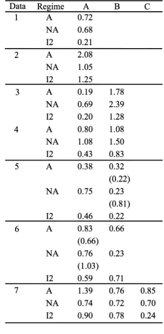
Table II summarizes the accuracy of extracted motion pa-rameters in terms of the MRE for each of the applied move-ments in the seven datasets. The majority of values were con-siderably less than 1 pixel. Generally, the MRE obtained after a second iteration of motion correction (I2) improved on the single-iteration value (A) as expected. There was no clear in-dication that including attenuation (A) gave consistently better motion estimates. The raw data (not shown) used to derive the MRE values indicated that all rotational and translational DOF were transparent to the algorithm. Maximum deviations from the applied values (across all optimizations) were 3.6 -(rota-tion), 4.2 -(rotation), 5.6 -(rotation), 1.8 mm ( ), 2.2 mm
TABLE II
MRES(PIXELS)FOR THEMOTIONESTIMATES IN THEDIGITAL
PHANTOMEXPERIMENTS
TABLE III
MEANABSOLUTEDEVIATION OFEXTRACTEDROTATIONS( )AND
TRANSLATIONS(PIXELS) FROMAPPLIEDPARAMETERS
( ), and 0.9 mm ( ). The mean absolute deviations
for each DOF and each correction regime are shown in Table III. These were similar using a single iteration with and without attenuation (A and NA, respectively) but were smaller in all DOF using a second iteration (I2). Moreover, the axis ro-tation was the most error-prone roro-tation parameter and the axis translation the most accurate translation parameter, irrespective of the correction regime used.
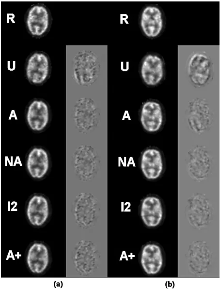
Fig. 6. Upper, middle, and lower (left to right) brain slices for (a) dataset 5 and (b) dataset 7. The three slices are shown for the free (R), motion-corrupted (U), and motion-corrected (A, NA, I2) reconstructions.
Fig. 7. (a) Dataset 5 and (b) dataset 7. A middle brain slice (left column) is shown for the motion-free (R), motion-corrupted (U), motion-corrected (A, NA, I2), and ideal-corrected(A ) reconstructions. Shown alongside each slice is the difference image formed by subtracting the motion-free slice. (Difference images were scaled to the same range.)
Only minor differences were apparent between correction regimes.
Fig. 7 repeats the vertical sequence of slices shown in Fig. 6, with the difference image between each slice and the motion-free counterpart shown alongside. The last row corresponds to the best-achievable correction (obtained using the known parameters). For dataset 5 [Fig. 7(a)],
dif-TABLE IV
MSDR VALUESAFTERMOTIONCORRECTION OF THESEVENDIGITAL
PHANTOMDATASETSUSINGEACHCORRECTIONREGIME
Fig. 8. Plot of MSDR values for each correction regime, expressed as a fraction of the MSDR for ideal(A ) correction.
ferences that were most obvious around the perimeter of the motion-corrupted slice were reduced by a similar extent using all correction regimes. For dataset 6 [Fig. 7(b)], distortions in the motion-corrupted slice were predominantly anterior and posterior. The bulk of these differences were removed by motion correction. A second iteration (I2) removed the postero-lateral difference still present after correction using regime A. These defects were removed using a single iteration without attenuation (NA). Clear residual differences existed after motion correction. However, the close resemblance between these difference images indicates that motion-induced distortions were reduced close to the potential of the technique. Noise and interpolation incurred between OSEM updates may be contributors to the residual error observed.
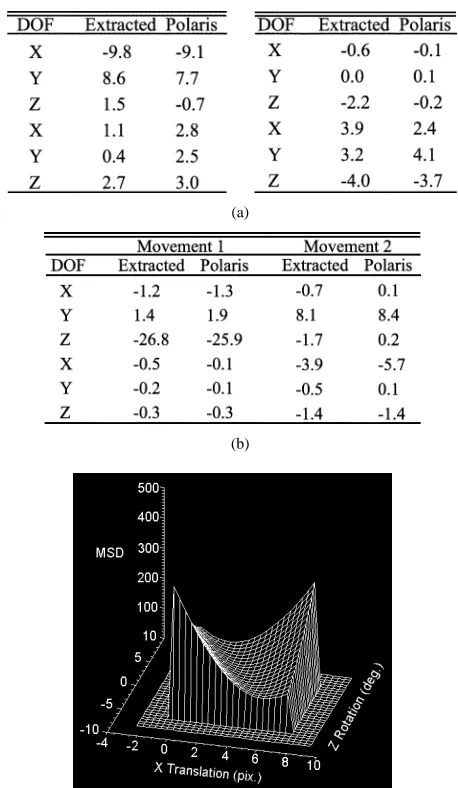
TABLE V
EXTRACTED ANDPOLARIS-MEASUREDROTATIONS( )ANDTRANSLATIONS
(PIXELS)FOR(a)THEFIRST(LEFT)ANDSECOND(RIGHT)
AND(b) THIRDPHYSICALPHANTOMDATASETS
(a)
(b)
Fig. 9. Surface plot of the similarity measure for one of the physical phantom datasets, showing a valley traversing the x-translation z-rotation parameter space. Shallowness made locating the minimum difficult and resulted in a discrepancy between the extracted and Polaris-measured values in some cases.
B. Physical Phantom
Table V shows the motion parameters extracted using the data-driven approach, and those measured by the Polaris motion tracker. For datasets 1 and 2 [Table V(a)] which had single corrupting movements, there was good agreement for three DOF ( and rotation, translation) and reasonable discrepancy for the remaining DOF ( and translation, rotation). Fig. 9 shows a surface plot of the similarity measure (C) as the -translational and -rotational parameters were manually driven through the range to pixels, and to , respectively (fixing the remaining parameters at the Polaris values). The topology shows there is difficulty in identifying the parameters corresponding to the minimum C value.
For dataset 3 [Table V(b)], there was much better agreement overall between the extracted parameters and Polaris parame-ters. Applying each set of parameters for motion correction re-sulted in the corrected slices shown in Fig. 10. Motion correction
Fig. 10. Upper, middle, and lower brain slices (left to right) shown for physical phantom dataset 3 (three head positions). The uncorrected study (U) had sig-nificant artifacts. Using the NA regime (NA) and Polaris measurements (P) for correction gave a very similar result, each significantly reducing the distortion.
gave significant improvement relative to the uncorrected slices. The similarity of the corrected slices suggests the data-driven motion correction was close to the best achievable in this case.
IV. DISCUSSION
The digital phantom results demonstrate that attenuation effects can be ignored in the motion estimation and updating stages of the algorithm. This regime achieved a level of correc-tion similar to two iteracorrec-tions with attenuacorrec-tion accounted for. Moreover, efficiency was approximately doubled since compu-tations related to transformation and projection of the attenuation map were bypassed. Although the results suggest further im-provement could be obtained from a second iteration without attenuation, we believe it preferable to retain the single-iteration speed advantage since the relative improvement from a second iteration would be small.
The digital phantom corrections confirmed the surprising ro-bustness of a partial reconstruction for optimization [18] even when only a small fraction of the data were utilized. In three datasets (5, 6, 7), less than angle pairs were used to form the partial reconstruction, yet corrections % of that achiev-able using the ideal motion parameters were obtained.
Discrepancy in some DOF for the Hoffman physical phantom experiments was due to a nearly flat region of the similarity function. We postulate that this behavior is a result of object symmetry not expected to be problematic in clinical data. An off-axis, axial rotation of a cylindrically symmetric, uniform ac-tivity distribution cannot be uniquely estimated using the pro-jection images. The physical phantom design allows activity to spread around the circular insert, leading to a hot rectangle of activity in the projection images. This possibly biases the esti-mation by confusing axial rotation with translational movement in the plane of projection.
slow, drifting motion that has been observed by some authors (e.g., [12] and [20]) can be approximated by a stepwise series of discrete movements as in dataset 7 (see Fig. 5). The overall accuracy of extracted results shows that this motion correction approach has the potential to rectify studies corrupted by com-plex movements, occurring at any stage in the acquisition, and of a magnitude typical of that observed clinically [4], [20].
Currently, only list-mode acquisition methods that bin data according to the location of the (tracked) brain are capable of fully correcting patient motion in SPECT since inter and in-traprojection motion is accounted for. We have shown previ-ously that our data-driven approach will correct the average movement within a projection [17]. However, it is clearly lim-ited when extensive motion occurs during projections.
It was assumed that the simplex algorithm would converge to a better solution if all angles corresponding to a particular brain position were included in the cost function. Under this as-sumption, identification of maximal-size motion groups is de-sirable. The method of applying arbitrary transformations to the reconstruction enabled such groups to be found in most datasets. For datasets 5 and 6 it was necessary to define one additional group. It is recognized that identification of large angle groups could be less likely if motion is slow and progressive. In terms of motion correction, this means more optimizations—the extreme case being a separate optimization for each angle pair/triple. For dual-head 90 camera geometry this in turn would require re-construction updates using subsets of two (angle pairs). Though OSEM may be limited here by the subset balance condition, the more general form of this iterative reconstruction algorithm, rescaled block iterative (RBI), should have no such limitation. Further investigation of this is required. In theory then, the iden-tification of angle groups is not a limitation, though at the cur-rent speed, failing to identify reasonably sized groups would make the algorithm prohibitively long to be practical.
An additional complicating factor when finding motion rela-tionships between angles is the choice of reconstruction subsets. For dataset 2, no motion groups were identifiable from the ini-tial comparison of acquired and forward-projected data since all subsets were equally weighted with moved and unmoved data. (However, arbitrarily transforming the reconstruction be-fore comparison did allow the two angle groups to be clearly identified.) Also, despite a smaller proportion of the study being corrupted, motion estimates were poorer than for some more significantly corrupted studies. In this case, the partial recon-struction was noticeably asymmetric due to the location of avail-able data. Further investigation is necessary into how influen-tial OSEM subset ordering is in distinguishing angle groups and estimating motion. Again, subset-based reconstruction al-gorithms not reliant on subset size or ordering may provide improvements.
V. CONCLUSION
A novel, 3-D motion correction technique for brain SPECT has been described that is relatively simple to implement. The method uses forward-projected data to determine brain motions and incorporates this information in a 3-D reconstruction. Arti-facts were reduced significantly in phantom data corrupted by single and multiple 3-D motions of varying magnitude and ex-tent. Specifically, a partial reconstruction should be used in
pref-erence to the full reconstruction to provide better estimates of brain movements. Attenuation can be ignored in the optimiza-tion stage and the bulk of mooptimiza-tion error is removed using a single iteration. Work is in progress to implement these findings in a clinical validation study.
ACKNOWLEDGMENT
The authors would like to acknowledge Dr. R. Fulton and Dr. M. Braun for their ideas and help in this work.
REFERENCES
[1] K. M. Silver, G. M. Currie, and A. F. McLaughlin, “Patient motion arte-fact characterization in cerebral SPECT acquisition,” A.N.Z. Nucl. Med., pp. 22–25, 1994.
[2] J. A. Cooper and B. K. McCandless, “Preventing patient motion during tomographic myocaridal perusion imaging,” J. Nucl. Med., vol. 36, pp. 2001–2005, 1995.
[3] E. H. Botvinick, Y. Y. Zhu, W. J. O’Connell, and M. W. Dae, “A quantita-tive assessment of patient motion and its effect on myocardial perfusion SPECT images,” J. Nucl. Med., vol. 34, pp. 303–310, 1993.
[4] M. V. Green, J. Seidel, S. D. Stein, T. E. Tedder, K. M. Kempner, C. Kertzman, and T. A. Zeffiro, “Head movement in normal subjects during stimulated PET brain imaging with and without head restraint,” J. Nucl.
Med., vol. 35, pp. 1538–1546, 1994.
[5] M. K. O’Connor, K. M. Kanal, M. W. Gebhard, and P. J. Rossman, “Comparison of four motion correction techniques in SPECT imaging of the heart: A cardiac phantom study,” J. Nucl. Med., vol. 39, pp. 2027–2034, 1998.
[6] G. Germano, T. Chua, P. B. Kavanagh, H. Kiat, and D. S. Berman, “De-tection and correction of patient motion in dynamic and static myocar-dial SPECT using a multi-detector camera,” J. Nucl. Med., vol. 34, pp. 1349–1355, 1993.
[7] G. Germano, P. B. Kavanagh, H. Kiat, K. Van Train, and D. S. Berman, “Temporal image fractionation: Rejection of motion artifacts in myocar-dial SPECT,” J. Nucl. Med., vol. 35, pp. 1193–1197, 1994.
[8] M. Ivanovic, D. A. Weber, S. Loncaric, C. Pellot-Barakat, and D. K. Shelton, “Patient motion correction for multicamera SPECT using 360 deg acquisition/detector,” Proc. IEEE Nuclear Science Symp., pp. 989–993, Nov. 1997.
[9] C. Pellot-Barakat, M. Ivanovic, D. A. Weber, A. Herment, and D. K. Shelton, “Motion detection in triple scan SPECT imaging,” IEEE Trans.
Nucl. Sci., vol. 45, pp. 2238–2244, Aug. 1998.
[10] S. R. Goldstein, M. E. Daube-Witherspoon, M. V. Green, and A. Eidsath, “A head motion measurement system suitable for emission computed tomography,” IEEE Trans. Med. Imag., vol. 16, pp. 17–27, Feb. 1997. [11] B. J. Lopresti et al., “Implementation and performance of an optical
motion tracking system for high resolution brain PET imaging,” IEEE.
Trans. Nucl. Sci., vol. 46, pp. 2059–2067, Dec. 1999.
[12] R. R. Fulton, “Correction for Patient Motion in Emission Tomography,” Ph.D. dissertation, Univ. Technol., Dept. Appl. Phys., Sydney, New South Wales, 2000.
[13] R. R. Fulton, B. F. Hutton, M. Braun, B. Ardekani, and R. Larkin, “Use of 3D reconstruction to correct for patient motion in SPECT,” Phys.
Med. Biol., vol. 39, pp. 563–574, 1994.
[14] R. R. Fulton, S. Eberl, S. R. Meikle, B. F. Hutton, and M. Braun, “A practical 3D tomographic method for correcting patient head motion in clinical SPECT,” IEEE Trans. Nucl. Sci., vol. 46, pp. 667–672, June 1999.
[15] L. K. Arata, P. H. Pretorius, and M. A. King, “Correction of organ mo-tion in SPECT using reprojecmo-tion data,” in IEEE Nuclear Science Symp.
Conf. Rec., 1996, pp. 1456–1460.
[16] K. J. Lee and D. C. Barber, “Use of forward projection to correct patient motion during SPECT imaging,” Phys. Med. Biol., vol. 43, pp. 171–187, 1998.
[17] B. F. Hutton, A. Z. Kyme, Y. H. Lau, D. W. Skerrett, and R. R. Fulton, “A hybrid 3D reconstruction/registration algorithm for correction of head motion in emission tomography,” IEEE Trans. Nucl. Sci., vol. 49, pp. 188–194, Feb. 2002.
[18] A. Z. Kyme, B. F. Hutton, R. L. Hatton, and D. W. Skerrett, “Optimizing data-driven motion correction in brain SPECT: Partial reconstruction and attenuation correction,” J. Nucl. Med., vol. 43, p. 222P, 2002. Abs. [19] H. M. Hudson and R. S. Larkin, “Accelerated image reconstruction using ordered subsets of projection data,” IEEE Trans. Med. Imag., vol. 13, pp. 601–609, Dec. 1994.