R E S E A R C H
Open Access
A method of 3D object recognition and
localization in a cloud of points
Jerzy Bielicki
*and Robert Sitnik
Abstract
The proposed method given in this article is prepared for analysis of data in the form of cloud of points directly from 3D measurements. It is designed for use in the end-user applications that can directly be integrated with 3D scanning software. The method utilizes locally calculated feature vectors (FVs) in point cloud data.
Recognition is based on comparison of the analyzed scene with reference object library. A global descriptor in the form of a set of spatially distributed FVs is created for each reference model. During the detection process, correlation of subsets of reference FVs with FVs calculated in the scene is computed. Features utilized in the algorithm are based on parameters, which qualitatively estimate mean and Gaussian curvatures. Replacement of differentiation with averaging in the curvatures estimation makes the algorithm more resistant to
discontinuities and poor quality of the input data. Utilization of the FV subsets allows to detect partially occluded and cluttered objects in the scene, while additional spatial information maintains false positive rate at a reasonably low level.
Keywords:3D object recognition, Point cloud
Introduction
Prevalence of 3D data acquisition optical systems demands development of dedicated algorithms for an efficient ana-lysis of such data in various fields of civil engineering, entertainment, and industry. Automated monitoring systems more and more often require end-user applications that are able to perform basic analysis or to detect unex-pected object presence or behavior. Monitoring of large amount of visual data (e.g., representing terrain after flood, hurricane or another natural catastrophe) to find predefined objects (e.g., human bodies or generally 3D objects) that may be only partially visible is a difficult task for people. It demands constant focus, which usu-ally varies in time. Efficiency of such analysis depends on human factor, and may lead to serious mistakes, that may cost human beings. Proposed method is suitable for such tasks due to automatic processing of large datasets, and specifying areas (with shape similar to requested; e.g., with higher probability than defined threshold), that should be analyzed precisely by human
operator (to avoid false-positive mistakes). Such a solu-tion allows to apply robust and automated analysis for whole dataset, while only the limited areas require more efficient and expensive analysis performed by well-trained human operator.
Most of the existing algorithms are based on either local or global object description. The local approach allows to effectively detect partially occluded objects. Utilization of 3D curves to describe edges of the objects and splashes to describe variations of surface normals within the local neighbourhood is described in [1]. Other local representations are point signatures (similar to splashes, but avoiding first-order derivative calculations) describing neighbour surface by analysis of sphere– surface intersections [2], point fingerprints (where geo-desic circles are projected onto surface tangent planes) [3], or keypoints with quality measure, based on values of principal curvatures (more sensitive to presence of noise and discontinuities, as it requires second-order derivative calculations) [4]. Locally based recognition is relatively fast, as it does not require computation of any features dependent on the size of the model. The disadvantage is that information provided only by a small part of the * Correspondence:[email protected]
Institute of Micromechanics and Photonics, Warsaw University of Technology, 8 Sw. Andrzeja Boboli, 02-525, Warsaw, Poland
object may easily be corrupted by, e.g., noise, and mis-lead the detection process.
The global approach may be less dependent on the local quality of analyzed surface. Utilization of oriented surface–point pair (point and surface normal at this point) histograms and review of their statistical compari-son criteria are presented in [5]. Other methods apply 3D modification of Hough transform for object similar-ity retrieval [6], or exploit reference object information from range image for efficient, low-level comparison implemented on GPU [7]. Important drawbacks include sensitivity to the loss of information (e.g., occlusion), misinformation (e.g., clutter) and time of data processing usually proportional to the object size.
Some existing algorithms require segmentation of the analyzed scene, which uses either a priori knowledge about input data or simple segmentation rules. Treating horizontally oriented planes as background to easily ex-tract objects [8], or clustering scene using distance-related feature [9] limits the generality of the algorithm. It often leads to under or over segmentation, what may result in significant errors, what is considered in the smoothness constraint segmentation problem [10].
Popular approach to 3D recognition problem is to exploit range images, also known as depth maps. These maps make data processing significantly faster, as they convert the most time-consuming problems (e.g., neigh-bourhood finding) from 3D into 2D space. Such a conver-sion into deeply studied image comparison problem allows to calculate more efficiently local surface descriptors (2D local histograms describing distribution of shape index [11] versus scanning angle) [12], to match multidimen-sional object histograms (distributions of surface normals and shape indexes) [13], or to focus on implementation of efficient algorithms directly on the GPU [7]. Interesting, but requiring preceding conversion from range image data into mesh model, is tensor-based representation of local surface patches, with voting scheme using 4D hash table [14]. However, the drawback of this approach is that it cannot analyze surfaces representing complete volumes. A range image is a projection of the single, directional point cloud (which is point cloud acquired from single direction—so-called 2.5D data) onto a plane, therefore uniqueness cannot be maintained for full 3D objects (formed from numerous directional clouds of points integrated in a single model).
Another approach converting 3D recognition problem into 2D image correlation task is to exploit spin-images, presented in [15,16]. Spin-image is a 2D accumulator located at oriented point (point with surface normal ns at this point), which collects all points, that are intersection of analyzed object and rectangle rotated around surface normal. Only such points are taken into consideration, which surface normals are deviated from surface normal
(ns) direction less than certain angle threshold. Such a solution is time-efficient regarding scene-model point matching. Drawback of this approach is the fact, that for optimal object description, setting the angle threshold requires knowledge about shape complexity of reference objects and objects analyzed in the scene.
Topology of the analysed data is exploited by another group of algorithms related to Non-rigid shapes [17], where statistical significance measure uses geodesic metrics as partial similarity criterion [18], or where 3D object is characterized by a set of signatures (histograms of geomet-ric distances, diffusion distances, the ratio of diffusion and geodesic distances, and two curvature-related histograms) which allows to determine similarity between objects as a multiplication of the pair wise histogram comparison (with χ2measure) results [19]. Unfortunately, they are not suitable for data in the form of single directional point clouds. Topology of an object represented by a directional point cloud may easily be changed due to the presence of noise or occlusion. This would intro-duce significant errors in the recognition process that use such type of algorithms.
optional, but in result significant operator support in critical situations.
Main text
Method
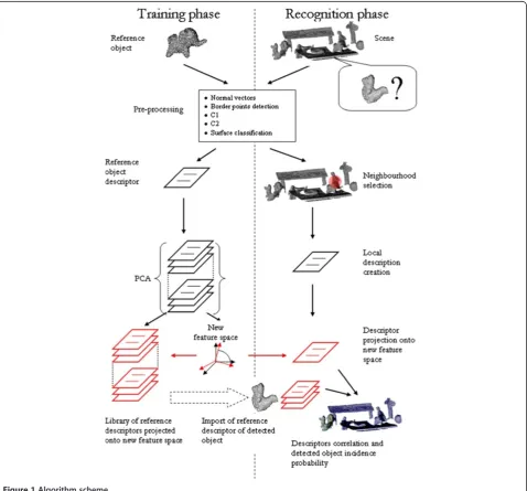
The proposed algorithm is divided into two phases (Figure 1). First is the training phase, performed off-line, when reference object database is created. Second phase is the recognition process, performed on-line. Both phases use common pre-processing (PP) in the beginning of the data processing flow. PP extracts geometrical features from the input data, which are utilized in the further steps. Detection results are presented as a probability distribu-tion of the object presence in the scene.
PP
First, the common stage of both phases of the proposed algorithm consists five steps, which are preceded by sim-ple point cloud average distance calculation to allow fur-ther automatic calculations on 3D input data.
Average point-to-point distance calculation
This step precedes PP and is used to estimate the aver-age distance between points in the input data. A set of random points (approximately 1000, or less if model is smaller than 1000 points) is selected and for each point the distance to the closest neighbour point is calculated and the average distance is found. It allows to set a value of neighbourhood radius rfor each calculation step as a multiplication of an average point distance, so it is not
necessary to know the dimensions of the measured objects. Value of neighbourhood radius is set arbitrary, assuring non-zero neighbourhood even in the presence of fluctu-ation of the local cloud density. In all calculfluctu-ations presented in the article neighbourhood radiusr= 6.
Data PP consists of following steps:
surface normal vectors estimation,
border points detection,
C1 parameter computation [26]
C2 parameter computation,
surface-type estimation.
Surface normal vectors estimation
In the next step, normal vectors for the directional point cloud data are calculated. For each point, a best fit plane (BFP) to the surface within the neighbourhood is estimated, using Root Mean Square (RMS) minimization criterion [27]. Obtained BFP is described by coefficientsA,B,Cand Din plane Equation (1). Normal vector is denoted as a set of normalized coefficients (A,B,C) from Equation (1), and its orientation is determined by the location of the scanning system (normal vector is oriented towards scanning system, which is equivalent toC> 0).
BFP:AxþByþCzþD¼0 ð1Þ
Border points detection
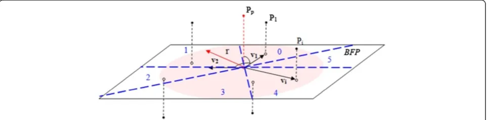
Surface of the BFP is radially divided into six equal zones (angle of each zone is approximately 60°) with the projection of currently analysed pointppused as division centre (Figure 2) [28]. BFP division is made using vector v1, which connects projections of the arbitrary neighbour point p1 with division centre pp, and using vector v2, which is a vector product of BFP normal and vector v1. Each zone accumulates orthogonal projections of every neighbour point pi onto the BFP. Lack of points in any of the zones indicates that the considered point belongs to an edge. Division orientation for each BFP is arbitrary,
but it does not affect the result of the border detection stage.
C1
ParameterC1 is defined as follows [26].
For each sampling point ppsigned, weighted, average distance to BFP is calculated. Distance with sign means that the sign of the value depends on the location of neighbour point pi with respect to the BFP normal vec-tor (Figure 3). Points located on the same side of the BFP as its normal vector contribute with positive value di whereas points on the opposite side contribute with negative value dj. Weightwi for each neighbour point is proportional to the Gaussian distribution of the distance si between orthogonal projections of sampling point pp
and neighbour point pi: wi∼e
s2i
2r2, where r is the neigh-bourhood radius. Value of C1 is greater than zero for convex surfaces, smaller than zero for concave surfaces and equal to zero for planes or saddle points.C1 param-eter corresponds qualitatively to mean curvature, which is arithmetical mean of main surface curvatures.
C2
ParameterC2 is defined as below [26].
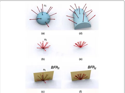
For each sampling pointpp, a best plane (BFPN) is fit-ted to all its neighbour normal vectors (such as ni), and average distance between BFPN and tips of the normal vectors is calculated (Figure 4c,f ). As one can see, for cylindrical surfaces (Figure 4d–f ) C2 value is equal to zero, while for spherical surfaces (Figure 4a–c) value of C2 is positive. Negative value ofC2 denotes saddle-like surface. For each neighbour point pi, inner product of normal ni and vector vi is also calculated. Vector vi connects orthogonal projections of sampling point pp and neighbour pointpionto BFP (Figure 5). Sign of each inner product vi ni gives information whether surface surrounding neighbourhood pointpiis concave or convex. Presence of noise can cause local fluctuations of direction of normal vectors and change sign of particular inner
products. Taking it into consideration, the presence of saddle-like surface is indicated when number of the inner products with opposite signs exceeds 35%.C2 parameter corresponds qualitatively to Gaussian curvature, which is a multiplication of main surface curvatures.
Local surface type
Local surface type is estimated using parameters C1 and C2 (Table 1). Positive signs of values of both parameters indicate convex ellipsoidal surface. Negative sign of C2 parameter value indicates that one of the main curvatures Figure 3C1 parameter estimation.C1 value is a signed, weighted average point distance to BFP, where weight is proportional to Gaussian function of point distancesiand neighbourhood radiusr.
is negative, which means that the surface is saddle-like. When C2 parameter value is zero, then surface is planar forC1 parameter equal to zero, and cylindrical otherwise. Sign of theC1 parameter then indicates cylinder convexity (or ellipsoid convexity for positiveC2 value). Local surface type corresponds to shape index introduced by Koenderink and van Doorn [11] utilized in [6,12,13], which is basically a mapping of main curvatures into polar system, where angle denotes the surface type, and distance from origin denotes the values of the curvatures. Shape index s is denoted with equation:
s¼2 πarctan
κ2þκ1
κ2κ1
ð2Þ
whereκ1andκ2are main curvatures. As it can be seen in Table 1, local surface type parameter can have eight differ-ent values, utilized in further calculations.
Training phase
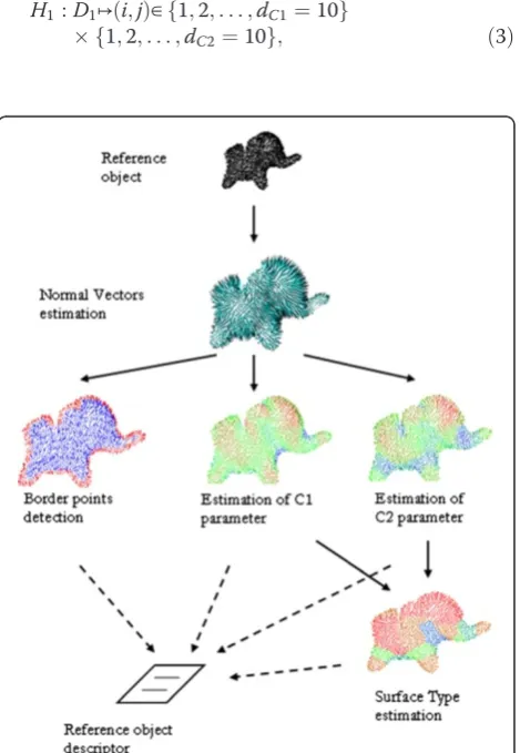
In this off-line phase, a description of the reference object is created. Based on the PP results the local feature vectors (FVs) are computed, and then collected to form a global descriptor for each reference object (Figure 6). Further, re-duction of the feature space dimensionality using principal component analysis (PCA) is performed [29].
Descriptor of a reference object consists of a set of local FVs, each of which is calculated for a sampling pointpn. Since the local FV is calculated for everynth point of the data, the number of FVs depends on sampling resolution of the reference model. The descriptor also contains the radius Rof the smallest bounding sphere for the model. The radius R is utilized in recognition phase to specify neighbourhood for local FV calculations.
Each local FV contains two histograms. First one is 2D distributionC1 versusC2 (Figure 7).
H1:D1↦ð Þ∈i;j f1;2;. . .;dC1¼10g
f1;2;. . .;dC2¼10g; ð3Þ
Figure 5Estimation of surface convexity.Positive inner product denotes convex surface, otherwise surface is concave.
Table 1 Local surface type estimation usingHandK (mean and Gaussian curvature, respectively) or usingC1 andC2 parameters, equivalently
Surface type H K C1 C2
Plane 0 0 0 0
Convex cylinder >0 0 >0 0
Concave cylinder <0 0 <0 0
Convex ellipsoid >0 >0 >0 >0
Concave ellipsoid <0 >0 <0 >0
Saddle-like surface >0 >0
=0 <0 =0 <0
where dC1 is a number of intervals for C1 distribution anddC2is a number of intervals forC2 distribution. The other one is a local surface type distribution:
H2:D2↦ð Þ∈i f1;2;. . .;dS¼8g ð4Þ
where dS is a number of intervals. Dimensionality of the feature spaceFSis thenN=dC1⋅dC2+dS. Each local FV contains also minimal and maximal values of parameters C1 andC2 and coordinates of the sampling point pn, for which the vector is calculated. During this process all edge points are ignored, as the information obtained for these areas may be misleading. For each local FV only the points located closer than 60% of radius R are considered. It implies that only approximately 30% of reference model surface is considered for a single FV and partial occlu-sion or clutter affects only few FVs. Due to this fact the algorithm is more resistant to these adverse conditions.
The last step of the training phase is PCA, which reduces dimensionality of the created feature space. Fea-ture space is reduced from initialN= 108 dimensions into significantly smaller space, usually less than 10D. Condi-tion taken into consideraCondi-tion during PCA is to preserve 99% of initial energy. It guarantees that only the most meaningful linear combinations of initial features will be considered in the recognition phase.
Recognition phase
In this on-line phase, scene-model matching is performed. Based on the PP results, local FV is created. Then the local FV is correlated with reference object descriptors. The thresholding step leads to the final decision about object presence.
Local model-scene correlation
The step following the PP stage is introduced to compute the local FV for each sampling point. Similarly to the
training phase, everynth point is sampled. The size of neigh-bourhood (denoted by the radiusR) utilized for the calcula-tion of local FVs depends on the size of the reference object that is looked for (see 1.2 paragraph for details). Each of the scene’s local FVs is projected onto feature spaceFS and then correlated with all FVs of the reference object. Correlation degree is denoted as a local probabilityPof object existence, and is calculated as follows:
P¼e kddrefk
2
dref
k k2
¼e
XN
o¼1ðdodroÞ 2
XN
o¼1dro 2
ð5Þ
whered = [d1,. . .,dN] is the projection of the localFVn onto feature space FS, dref = [dr1,. . .,drN] is the projec-tion of one of the reference model’s localFVklonto fea-ture spaceFS.
As a result a set of probability distributionsPiklis obtained, whereiis point index,kis the index of the reference object andlis the index of one of the reference model’s localFVkl.
Thresholding
At this stage, final decision about the presence of one or multiple objects is made. Sensitivity of the algorithm is modified using three parameters:
Tp – probability threshold; all points with probability
PiklbelowTpare ignored,
Dp–distance difference threshold; a pair of scene sam-pling points is accepted only if the difference between dis-tance |Pi Pj| and |Pkl Pkm| is smaller than the threshold value, where |Pi Pj|–distance between neighbour points
pi and pj, with probabilities Pikl and Pjkm, respectively, |PklPkm|– distance between reference object sampling pointspklandpkm, for which localFVkl andFVkmwere calculated.
Np–number of accepted points threshold; forNp= 3 similar triangles, and forNp= 4 similar quadrangles, are searched.
Thresholding algorithm (Figure 8) is shown below.
1. Pointp1with probabilityP1klhigher thanTpis searched. If found,k(object index) andl(FV index) are remembered (Figure8a).
2. Pointp2with probabilityP2kmhigher thanTpis searched. Additional condition to satisfy is
jjp1p2j jpklpkmjj<Dp⋅jpklpkmj for l≠m ð6Þ
which corresponds to the fact that a line segment |PiPj| similar to the reference model segment |PklPkm| is found in the scene (Figure8b).
3. IfNp= 3, then last, third pointp3is searched. That point has to satisfy condition (6) against both points
p1andp2(Figure8c). To guarantee similarity between detected and referenced triangle, direction of vector product in relation to average direction of normal vectors is checked. If succeeded, a triangle similar to the triangle from reference model is found in the scene and average probability is calculated. If Np= 4, a fourth point is searched to find a similar
quadrangle. All probabilities are sorted top to bottom, so even if the search does not succeed, performance of the algorithm is high.
At the end of the recognition phase all small, adjacent groups of selected points are converted into consistent objects.
Results
Assessment of the proposed method was performed using synthetic and real input data. Synthetic data have mostly been used to evaluate the influence of data quality on de-tection results. Real data were captured using the OGX| 3DMADMACscanner [30,31].
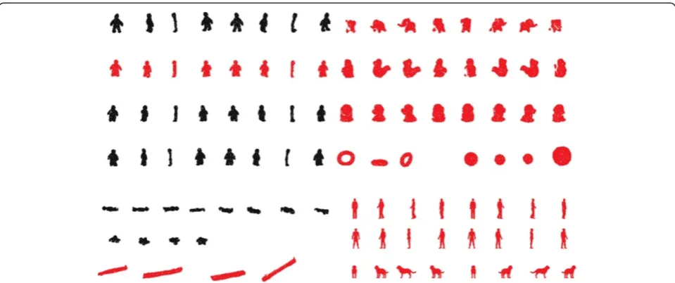
For the purpose of algorithm evaluation, an object data-base was created (red objects in Figure 9). Each reference object is presented as a set of directional point clouds
acquired from various points of view. Direction of data acquisition changes horizontally. Angles between any two adjacent scans are approximately 45°. All objects apart from two human figures and a dog, located right bot-tom in Figure 9, were scanned with OGX|3DMADMAC scanner. Human figures and the dog are imported from Princeton Shape Benchmark (called further: human 1 PSB, human 2 PSB, dog PSB) [32], re-sampled and converted into directional point cloud to maintain consistency within input data. Conversion from full 3D model usually properly imitates point surface acquired during scanning process. If a 3D model consists of a set of volumes (i.e., computer designed model as a set of sub volumes), then created sur-face may be similar to one that has poor quality, but still allows to perform the calculation. All presented results (Figures 10, 11, 12) are made using colour map with red colour denoting probability close to 100%, through green denoting 50% to blue colour denoting 0%. Grey colour denotes probability below threshold.
figures, (d) elephant, (e) dinosaur and (f) dog. All objects apart from the plasticine figures are detected with prob-ability of nearly 100%. Plasticine figures are detected with lower, 80–90% probabilities. It is important to notice that only one of these figures was scanned as a reference object, and that all the figures differ from each other in shape, as they were hand-made.
Figure 11 shows one of the worst case detection results for (a) torus, (b) ball, (c) plasticine figures, (d) elephant, (e) dinosaur and (f ) dog. Figure 11a,c,d shows that in some cases local descriptors may not be descrip-tive enough to distinguish between similar objects. On the other hand, such a property reduces algorithm sensi-tivity to clutter and occlusion.
In Figure 12, a synthetic scene is presented. All the complex objects, such as (a) Porsche, aircraft and (b–d) Mercedes models have been converted from full 3D models (composed of multiple solids), so the obtained surfaces may locally be confusing for the algorithm. In Figure 12c, detec-tion of the dog PSB is presented. Figure 12a,b,d presents detection results of human 1 PSB. Figure 12b,d shows the influence of distance difference threshold Dp value on detection results for probability threshold Tp= 90%. For Figure 12b, withDp= 0,04 only the standing pose is detected. Increasing parameter value toDp= 0,1 results in detection of both human figures and in one false positive detection (Figure 12d). It can be seen that presence of obstacles in the neighbourhood does not Figure 9Reference objects database.Object marked as black (plasticine figurines) are not present in the created library.
strongly affect detection, since local descriptors are utilized. From the other hand it is noticeable that, with constant value of Dpthreshold, the bigger is maximum distance between reference points (which is a result of value of radius R of the analysed neighbourhood— see 1.2 for details) the bigger is tolerance field for real dif-ference between redif-ference points distance and candidate points distance. For better performance, value of Dp threshold should vary as a function of distance, to avoid linear increase of distance difference toleration with in-crease of the distance between reference points.
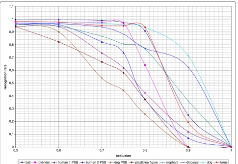
Figure 13 presents the relation of recognition rate versus occlusion for all the analysed objects. For most of the objects recognition rate above 80% is reached for 70% occlusion, since detection process utilizes a combin-ation of a small number of local FVs. Simultaneously, spatial information (analysis of distribution of at least three descriptors for each reference object) allows to keep false positive ratioat a reasonably low level. The achieved
results show that the proposed algorithm is resistant to occlusion. More sensitive to clutter and occlusion seem to be the algorithms, based on histogram comparison [5], where incompleteness of data may change comparison result significantly. Better performance present algorithms based on keypoints [4] with further ICP-type surface regis-tration, what may be less effective, when considering objects, that are in general similar, but differ from each other on the whole surface (i.e., plasticine figures), which is the most common case in real environment.
Robustness to clutter results from the fact that varying number of points representing other objects/background does not affect the locally calculated FVs, nor the detec-tion results. Nevertheless, the impact of spatial distribu-tion of clutter points is not easy to estimate.
Another important factor to consider is noise. Presence of the noise was simulated by adding to each object (syn-thetic or real) randomly generated noise of increasing amplitude. To maintain consistency within all reference Figure 11Recognition results in scenes scanned with OGX|3DMADMAC system.
objects, amplitude value depends on object’s diameter. Values of all detection parameters are the same as in pre-vious assessments. Influence of the noise on recognition efficiency is presented in Figure 14. Most of the objects are recognized with efficiency above 75% for amplitude noise reaching 5% of object diameter. Presence of noise seems to be crucial for descriptiveness of histograms presented in [5], as they require whole data of good quality for proper representation of the object. Sensitive to the presence of noise appear to be also point fingerprint ap-proach [3], as it utilizes geodesic curves, which length and position may strongly be disrupted by noisy points. For the ICP-type algorithms [4], presence of noise may slightly increase RMS error value (quality of surface registration), but should not strongly affect recognition rate.
The worst case presented in Figure 14 is recognition of the dog PSB. The reason seems to be the fact that even small amplitude noise added to, e.g., thin legs of the dog changes rapidly their shape (two legs may be joined into a single one). The next to the worst case is the cylinder. In this case, poor recognition result is caused by high ratio between length and radius of the cylinder. Large length implies high amplitude of random
noise, which, compared with small radius, significantly modifies the shape of the object. The rest of the objects are detected efficiently and increasing noise amplitude decreases the recognition accuracy at an acceptable rate. Utilization of the BFPs instead of spatial derivatives in the process of local surface type estimation improves algorithm’s resistance to noise or discontinuities within the input data.
Conclusion
In this article, efficient and robust to noise algorithm have been presented. Performed comparisons in the rec-ognition process are based on an approach avoiding noise-sensitive calculations, to make an algorithm suit-able for low-quality data. The assumption was to exploit minimum number of parameters, which completely de-scribe local geometry of the surface. Main step of the al-gorithm is to consider set of spatially distributed surface parts as a representation of reference object stored in database. Such an approach should allow to detect even strongly occluded objects, where detection is a result of finding similar structure during scene-model correlation process. Thanks that there is no significant difference
0 0,1 0,2 0,3 0,4 0,5 0,6 0,7 0,8 0,9 1 1,1
0,8 0,7
0,6 0,5
occlusion
re
c
ognition r
a
te
ball cylinder human 1 PSB human 2 PSB dog PSB plasticine figure elephant dinosaur dog torus
1 0,9
for the algorithm between occlusion and clutter, as long as noise is not similar in shape to the missing parts of detected objects.
Main drawback is, in some cases, descriptiveness of the proposed descriptor, which may result in high false posi-tive ratio. It may need to be minimized by improvements of geometrical representation of the reference object, and by utilizing quadrangles instead of triangles in thresholding process.
The results show that the proposed algorithm can be used with incomplete and noisy data. Impact of clutter on the recognition rate is also minimized because of the utilization of local FVs.
In the future, a sampling algorithm similar to Farthest Point Sampling[33] will be implemented to assure uniform data sampling. Also modification of the spatial representa-tion of the reference objects may improve descriptiveness and thanks to that reduce false positive recognition ratio. The most promising seems to be an implementation of two-level hierarchy model representation, which will be suitable for high detailed and point dense objects. At the moment, thresholding process results in finding in scene a triangle (or quadrangle), where its vertexes represent sur-face parts similar to the sursur-face of reference object. Adding top level hierarchy, resulting in detection of “triangle of triangles”of similar surface parts, will increase the accuracy of detection, especially of large models (i.e. huge animals)
which consist high detailed elements (i.e. head, legs, tail) which may be significant for distinction one from another (i.e. horse from rhinoceros). Another advantage of proposed modification is that it can represent each object as a spatial distribution of basic shapes, which is much more intuitive and easy to analyse for humans, than, i.e. set of keypoints [4], spin-images [16] or histograms [5], and can further be exploited in more abstract way (i.e. cognitive systems). Calculation time should not increase significantly, as the number of the most time-consuming calculations (scene-model similarity comparison) remains same, with change of the thresholding process only.
One of the advantages is that the same algorithm can add reference objects to the existing database, which allows to develop such a database whenever it is necessary. Presented method may efficiently assist the operators of the automated maintenance monitoring systems.
Competing interests
The authors declare that they have no competing interests.
Received: 12 February 2012 Accepted: 28 January 2013 Published: 21 February 2013
References
1. GM Fridtjof, Stein, Structural indexing: efficient 3-D object recognition. IEEE Trans. Pattern Anal. Mach. Intell.14(2), 125–145 (1992)
2. RJ Chin, Seng Chua, Point signatures a new representation for 3D object recognition. Int. J. Comput. Vis.25(1), 63–85 (1997)
0 0,1 0,2 0,3 0,4 0,5 0,6 0,7 0,8 0,9 1 1,1
0 1 2 3 4 5 6 7 8 9 10 11
noise ,% object diameter
re
cognition r
a
te
ball cylinder human 1 PSB human 2 PSB dog PSB plasticine figure elephant dinosaur dog torus
3. JP Yiyong Sun, K Andreas, DL Page, MA Abidi, The point fingerpint. A new 3-D object representation scheme. IEEE Trans. Syst. Man Cybern.33(4), 712–717 (2003) 4. A Mian, M Bennamoun, R Owens, On the repeatability and quality of
keypoints for local feature-based 3D object retrieval from cluttered scenes. Int. J. Comput. Vis.89, 348–361 (2009)
5. E Wahl, U Hillenbrand, G Hirzinger, Surflet-pair-relation histograms: a statistical 3D-shape representation for rapid classification, inProc. Fourth International Conference on 3-D Digital Imaging and Modeling, 2003, pp. 474–481 6. T Zaharia, F Preteux, Hough transform-based 3D mesh retrieval. Proc. SPIE
4476, 175–185 (2001)
7. MDB Marcel Germann,Automatic Pose Estimation for Range Images on the GPU(Hanspeter Pfister, Kyu Park, 2005)
8. RB Rusu, A Holzbach, M Beetz, G Bradski, Detecting and segmenting objects for mobile manipulation, inProc. IEEE 12th International Conference on Computer Vision Workshops, 2009, pp. 47–54
9. K Klasing, A clustering method for efficient segmentation of 3D laser data, inProc. IEEE International Conference on Robotics and Automation, 2008, pp. 4043–4048 10. T Rabbani, FA van den Heuvel, G Vosselman, Segmentation of point clouds
using smoothness constraint. ISPRSXXXVI(5), 248–253 (2006)
11. JJ Koenderink, AJ van Doorn, Surface shape and curvature scales. Image Vis. Comput.10(8), 557–564 (1992)
12. BB Hui, Chen, 3D free-form object recognition in range images using local surface patches. Pattern Recognit. Lett.28(10), 1252–1262 (2007) 13. B Leibe, G Hetzel, P Levi, B Schiele, 3D object recognition from range
images using local feature histograms, inProc. CVPR(II), 2001, pp. 394–399 14. AS Mian, M Bennamoun, RA Owens, 3D recognition and segmentation of
objects in cluttered scenes, inProc. ACV, 2005, pp. 8–13
15. E Andrew, MH Johnson, Surface matching for object recognition in complex 3-D scenes. Image Vis. Comput.16, 635–651 (1998)
16. E Andrew, MH Johnson, Using spin images for efficient object recognition in cluttered 3D scenes. IEEE Trans. Pattern Anal. Mach. Intell.21(5), 433–449 (1999) 17. M Ovsjanikov, Q-X Huang, L Guibas, A condition number for non-rigid
shape matching. Computer Graphics Focum30(5), 1503–1512 (2011) 18. AM Bronstein, MM Bronstein, Y Carmon, R Kimmel,Partial Similarity of
Shapes Using a Statistical Significance Measure(Department of Computer Science, Technion Israel Institute of Technology, Haifa, 2009) 19. M Mahmoudi, G Sapiro, Three-dimensional point cloud recognition via
distributions of geometric distances. Graphical Models71(1), 22–31 (2009) 20. J Goldfeather VI, A novel cubic-order algorithm for approximating principal
direction vectors. ACM Trans. Graph23, 45–63 (2004)
21. A Mustafa, L Shapiro, M Ganter, 3D object identification with color and curvature signatures. Pattern Recognit.32, 339–355 (1999)
22. A Colombo, C Cusano, R Schettini, 3D face detection using curvature analysis. Pattern Recognit.39, 444–455 (2006)
23. P Szeptycki, M Ardabilian, L Chen, A coarse-to-fine curvature analysis-based rotation invariant 3D face landmarking, inProc. International Conference of Biometrics: Theory, Applications and Systems, 2009, pp. 1–6
24. F Crosilla, D Visintini, F Sepic, Reliable automatic classification and segmentation of laser point clouds by statistical analysis of surface curvature values. Appl. Geomat.1(1–2), 17–30 (2009)
25. C Li, D Shaonyi, Z Nanning, A fast multi-resolution iterative closest point algorithm, inProc. CCPR, 2010, pp. 1–5
26. M Witkowski, R Sitnik, Locating and tracing of anatomical landmarks based on full-field four-dimensional measurement of human body surface. J. Biomed. Opt.13(4), 044039 (2008)
27. A Björck,Numerical Methods for Least Squares Problems(SIAM, Philadelphia, 1997) 28. E Kalogerakis, D Nowrouzezahrai, S Patricio, S Karan, Extracting lines of
curvature from noisy point clouds. Elsevier J. Comput.-Aided Design41
(Special Issue on Point-Based Computational Techniques), 282–292 (2009) 29. IT Jolliffe,Principal Component Analysis, 2nd edn. (Springer, New York, 2002) 30. R Sitnik, M Kujawińska, J Woźnicki, Digital fringe projection system for large-volume 360-deg shape measurement. Opt. Eng.443(41), 443–449 (2002) 31. OGX|Optographx. http://ogx.mchtr.pw.edu.pl/projects/3dmadmac/ 32. Princeton Shape Benchmark. http://shape.cs.princeton.edu/benchmark/ 33. AM Bronstein, MM Bronstein, R Kimmel,Numerical Geometry of Non-Rigid
Shapes(Springer Verlag, New York, 2009)
doi:10.1186/1687-6180-2013-29
Cite this article as:Bielicki and Sitnik:A method of 3D object recognition and localization in a cloud of points.EURASIP Journal on Advances in Signal Processing20132013:29.
Submit your manuscript to a
journal and benefi t from:
7 Convenient online submission 7 Rigorous peer review
7 Immediate publication on acceptance 7 Open access: articles freely available online 7 High visibility within the fi eld
7 Retaining the copyright to your article