A family of variable step-size affine projection adaptive filter algorithms using statistics of channel impulse response

R E S E A R C H

Open Access

A family of variable step-size affine projection

adaptive filter algorithms using statistics of

channel impulse response

Mohammad Shams Esfand Abadi

and Seyed Ali Asghar AbbasZadeh Arani

Abstract

This paper extends the recently introduced variable step-size (VSS) approach to the family of adaptive filter algorithms. This method uses prior knowledge of the channel impulse response statistic. Accordingly, optimal step-size vector is obtained by minimizing the mean-square deviation (MSD). The presented algorithms are the VSS affine projection algorithm (VSS-APA), the VSS selective partial update NLMS (VSS-SPU-NLMS), the VSS-SPU-APA, and the VSS selective regressor APA (VSS-SR-APA). In VSS-SPU adaptive algorithms the filter coefficients are partially updated which reduce the computational complexity. In VSS-SR-APA, the optimal selection of input regressors is performed during the adaptation. The presented algorithms have good convergence speed, low steady state mean square error (MSE), and low computational complexity features. We demonstrate the good performance of the proposed algorithms through several simulations in system identification scenario.

Keywords:Adaptive filter, Normalized Least Mean Square, Affine projection, Selective partial update, Selective regressor, Variable step-size

1. Introduction

Adaptive filtering has been, and still is, an area of active research that plays an active role in an ever increasing number of applications, such as noise cancellation, chan-nel estimation, chanchan-nel equalization and acoustic echo cancellation [1,2]. The least mean squares (LMS) and its normalized version (NLMS) are the workhorses of adap-tive filtering. In the presence of colored input signals, the LMS and NLMS algorithms have extremely slow conver-gence rates. To solve this problem, a number of adaptive filtering structures, based on affine subspace projections [3,4], data reusing adaptive algorithms [5,6], block adap-tive filters [2] and multi rate techniques [7,8] have been proposed in the literatures. In all these algorithms, the selected fixed step-size can change the convergence and the steady-state mean square error (MSE). It is well known that the steady-state MSE decreases when the step-size decreases, while the convergence speed increases when the step-size increases. By optimally selecting the step-size during the adaptation, we can

obtain both fast convergence rates and low steady-state MSE. These selections are based on various criteria. In [9], squared instantaneous errors were used. To improve noise immunity under Gaussian noise, the squared auto-correlation of errors at adjacent times was used in [10], and in [11], the fourth order cumulant of instantaneous error was adopted.

In [12], two adaptive step-size gradient adaptive filters were presented. In these algorithms, the step sizes were changed using a gradient descent algorithm designed to minimize the squared estimation error. This algorithm had fast convergence, low steady-state MSE, and good performance in nonstationary environment. The blind adaptive gradient (BAG) algorithm for code-aided sup-pression of multiple-access interference (MAI) and nar-row-band interference (NBI) in direct-sequence/code-division multiple-access (DS/CDMA) systems was pre-sented in [13]. The BAG algorithm was based on the concept of accelerating the convergence of a stochastic gradient algorithm by averaging. The authors shown that the BAG had identical convergence and tracking properties to recursive least squares (RLS) but had a computational cost similar to the LMS algorithm. In

* Correspondence: [email protected]

Faculty of Electrical and Computer Engineering, Shahid Rajaee Teacher Training University, Tehran, Iran

[14], two low complexity variable step size mechanisms were proposed for constrained minimum variance (CMV) receivers that operate with stochastic gradient algorithms and are also incorporated in the channel estimation algorithms. Also, the low low-complexity variable step size mechanism for blind code-constrained constant modulus algorithm (CCM) receivers was pro-posed in [15]. This approach was very useful for nonsta-tionary wireless environment.

In [16], a generalized normalized gradient descent (GNGD) algorithm for linear finite-impulse response (FIR) adaptive filters was introduced that represents an extension of the NLMS algorithm by means of an addi-tional gradient adaptive term in the denominator of the learning rate of NLMS. The simulation results show that the GNGD algorithm is robust to significant varia-tions of initial values of its parameters.

Important examples of two new variable step-size (VSS) versions of the NLMS and the affine projection algorithm (APA) can be found in [17]. In [17], the step-size is obtained by minimizing the mean-square deviation (MSD). This introduced algorithms show good performance in convergence rate and steady-state MSE. This approach was successfully extended to selective partial update (SPU) adaptive filter algorithm in [18].

To improve the performance of adaptive filter algo-rithms, the adaptive filter algorithm was proposed based on channel impulse response statistics [19,20]. In [21] a new variable-step-size control was proposed for the NLMS algorithm. In this algorithm, the step-size vector with different values for each filter coefficient was used. In this approach, based on prior knowledge of the channel impulse response statistics, the optimal step-size vector is obtained by minimizing the mean-square deviation (MSD) between the optimal and estimated filter coefficients.

Another feature which is important in adaptive filter algorithms is computational complexity. Several adaptive filters with fixed step-size, such as the adaptive filter algorithms with selective partial updates have been pro-posed to reduce the computational complexity. These algorithms update only a subset of the filter coefficients in each time iteration. The Max-NLMS [22], the variants of the SPU-NLMS [23], and SPU-APA [24,25] are important examples of this family of adaptive filter algo-rithms. Recently an affine projection adaptive filtering algorithm with selective regressors (SR) was also proposed to reduce the computational complexity of APA [26-28]. In this algorithm, the recent regressors are optimally selected during the adaptation.

In this paper, we extend the approach in [21] to the APA, SPU-NLMS, SPU-APA, and SR-APA and four novel VSS adaptive filter algorithms are established. These algorithms are computationally efficient.

We demonstrate the good performance of the presented algorithms through several simulation results in system identification scenario. The comparison of the proposed algorithms with other algorithms is also presented.

What we propose in this paper can be summarized as follows:

•The establishment of the VSS-APA.

•The establishment of the VSS-SPU-NLMS.

•The establishment of the VSS-SPU-APA.

•The establishment of the VSS-SR-APA.

•Demonstrating of the proposed algorithms in sys-tem identification scenario.

•Demonstrating the tracking ability of the proposed algorithms.

We have organized our paper as follows. In section 2, the NLMS and SPU-NLMS algorithms will be briefly reviewed. Then, the family of APA, SR-APA and SPU-APA are presented and the family of variable step-size adaptive filters is established. In the following, the computational complexity of the VSS adaptive filters is discussed. Finally, before concluding the paper, we demonstrate the usefulness of these algorithms by pre-senting several experimental results.

Throughout the paper, the following notations are adopted:

|.| norm of a scalar

||.||2squared Euclidean norm of a vector (.)Ttranspose of a vector or a matrix tr(.) trace of a matrix

E[.] expectation operator

2 Background on family of NLMS algorithm 2-1 Background on NLMS

The outputy(n) of an adaptive filter at timenis given by

y(n) =wT(n)X(n) (1)

wherew(n) = [w0(n),w1(n), ...,wM-1(n)]Tis theM × 1 filter coefficients vector andX(n) = [x(n),x(n-1), ..., x(n-M+1)]Tis the M× 1 of input signal vector. The NLMS algorithm is derived from the solution of the following constrained minimization problem [1]

min

w(n+1)w(n+ 1)−w(n) 2

Subject to wT(n+ 1)X(n) =d(n)

(2)

where d(n) is the desired signal. The resulting NLMS algorithm is given by the recursion

w(n+ 1) =w(n) + μ

whereμis the step-size which is introduced to control the convergence speed (0 <μ < 2). Also, e(n) is the output error signal which is defined as

e(n) =d(n)−y(n) (4)

2-2 Selective Partial Update NLMS

By partitioning the filter coefficients and input signal vec-tors to theBblocks each of lengthL(note thatB=M/L and is an integer),X(n) = [x1(n),x2(n), ...,xB(n)]Tandw(n) = [w1(n),w2(n), ...,wB(n)]T, the SPU-NLMS algorithm for a single block update at every iteration minimizes the following optimization problem:

min

wF(n+1)wF(n+ 1)−wF(n) 2

Subject to wT(n+ 1)X(n) =d(n)

(5)

where F = {j1, j2, ..., jS} denote the indices of the S blocks out of Bblocks that should be updated at every adaptation and wF(n) =

wj1,wj2, ...,wjS T

[24]. Again by using the method of Lagrange multipliers, and defining

XF(n) =

xj1(n),xj2(n), ...,xjS(n) T

, the update equation for SPU-NLMS is given by:

wF(n+ 1)=wF(n) + μ

XF(n)2XF(n)e(n)

Indices of F correspond to S largest values ofxj(n)2for1≤j≤B

(6)

ForM=BandL= 1, the SPU-NLMS algorithm in (6) reduces to

wi(n+ 1)=wi(n) + μ

x(n−i)e(n)

i=arg max

0≤j≤M−1|x(n−j)|

(7)

which is the max-NLMS algorithm [22]. ForM =B andL=B, the SPU-NLMS algorithm becomes identical to NLMS algorithm in (3).

3. Background on APA, SR-APA and SPU-APA 3-1. Affine projection algorithm (APA)

Now, define theM×Kmatrix of the input signal andK × 1 of the desired signal as:

X(n) = ⎡ ⎢ ⎣

x(n) . . . x(n−K+ 1) ..

. . .. ...

x(n−M+ 1). . .x(n−K−M+ 2) ⎤ ⎥

⎦ (8)

d(n) =d(n), ...,d(n−K+ 1)T (9)

whereKis a positive integer (usually, but not necessa-rily K≤ M). The family of APA can be established by minimizing relation (2) but subject tod(n) =XT(n)w(n +1). Again, by using the method of Lagrange multipliers, the filter vector update equation for the family of APA is given by:

w(n+ 1) =w(n) +μX(n)XT(n)X(n)−1e(n) (10) wheree(n) = [e(n),e(n-1), ...,e(n-K+1)]Tis the output error vector, which is defined as:

e(n) =d(n)−XT(n)w(n) (11)

3-2 Selective Regressor APA (SR-APA)

In [26], another novel affine projection algorithm with selective regressors (SR), called (SR-APA), was pre-sented. In this section, we briefly review the SR-APA. The SR-APA minimizes relation (2) subject to:

dG(n) =XTG(n)w(n+ 1) (12)

where G= {i1, i2, ..., ip} denote the P subset (subset withPmember) of the set {0, 1, ...,K-1}.

XG(n) =

⎡ ⎢ ⎣

x(n−i1) . . . x(n−ip)

..

. . .. ...

x(n−M+ 1−i1). . .x(n−M+ 1−ip)

⎤ ⎥ ⎦ (13)

is the M×Pmatrix of the input signal and:

dG(n) =

d(n−ii), ...,d

n−ip T

(14)

is the P × 1 vector of the desired signal. Using the method of Lagrange multipliers to solve this optimiza-tion problem leads to the following update equaoptimiza-tion:

w(n+ 1) =w(n) +μXG(n)

XT_G(n)XG(n) −1

eG(n) (15)

where

eG(n) =dG(n)−XTG(n)w(n) (16)

The indices of G are obtained by the following procedure:

1. Compute the following values for 0≤i≤K- 1:

e2(n−i)

X(n+i)2 (17)

3-3. Selective Partial Update APA (SPU-APA)

The SPU-APA solves the following optimization pro-blem [24]:

min

wF(n+1)wF(n+ 1)−wF(n) 2

Subject toXT(n)w(n+ 1) =d(n)

(18)

where F = {j1, j2, ..., jS} denote the indices of the S blocks out of Bblocks that should be updated at every adaptation. Again, by using the Lagrange multipliers approach, the filter vector update equation is given by:

wF(n+ 1) =wF(n) +μXF(n)

XT_F(n)XF(n) −1

e(n) (19)

where

XF(n) =

XT_j1(n),X_jT₂(n), ...,XT_js(n)T (20)

is theSL×Kmatrix and:

Xi(n) =

xi(n),xi(n−1), ...,xi(n−K+ 1)

(21)

is theL×Kmatrix. The indices of Fare obtained by the following procedure:

1. Compute the following values for 1≤i≤B:

TrX_iT(n)Xi(n)

(22)

2. The indices ofFcorrespond to S largest values of relation (22).

4. VSS-NLMS and the proposed VSS Adaptive Filter Algorithms

4-1. Variable Step-Size NLMS algorithm using statistics of channel response

Consider a linear system with its input signalX(n) and desired signald(n) are related by

d(n) =hTX(n) +v(n) (23)

whereh= [h0,h1, ...,hM-1]Tis the true unknown system with memory lengthM,X(n) = [x(n), ...,x(n-M+1)]Tis the system input vector, andv(n) is the additive noise.

The filter coefficients of VSS-NLMS are updated by [21]

w(n+ 1) =w(n) +U(n)X(n)e(n)

X(n)2 (24)

where the step-size matrix is defined asU(n) =diag[μ0 (n), ...,μM-1(n)].

To quantitatively evaluate the mis-adjustment of the filter coefficients, the MSD is taken as a figure of merit, which is defined as

(n) =E

w(n)2

(25)

where the weight error vector is given by

w(n) =w(n)−h (26)

Note that at each iteration, the MSD depends onμi(n), and by using the independent and identically distributed (i.i.d) sequence for input signal, we have

(n+ 1)≈1 +tr[U 2_(n)]

M2

Ew(n)2₋2 ME

wT_{(n)U(n)w(n)+trU}2_(n) σv2 M2_σ2

x (27)

The optimal step-size is obtained by minimizing the MSD at each iteration. Taking the first-order partial derivative ofΛ(n+1) with respect toμi(n)(i= 0, ..., M-1), and setting it to zero, we obtain

μi(n)=

MEw2

i(n)

Ew(n)2+σ 2

v

σ2

x

(28)

and

E[w2i(n+ 1)] =

1−2μi(n)

M

E[w2i(n)] +

μ2

i(n)

M2_σ2 x

E[e2(n)] (29)

We can estimate E[e2(n)] by a moving average approach ofe2(n):

σ2

e(n) =λσe2(n−1) + (1−λ)e2(n) (30)

where 0 < l < 1 is the forgetting factor. Also, the initial value for Ew2_i(0) is given by the second-order statistics of the channel impulse response, i.e. Eh2

i

.

4-2. Variable Step-Size Selective Partial Update NLMS algorithm using statistics of channel response The filter coefficients in SPU-NLMS are updated by

wF(n+ 1) =wF(n) +

UF(n) XF(n)2

XF(n)e(n)

where UF(n) =

μj1(n),μj2(n), ...,μjS(n) T

.

(31)

Approximatinge(n) with

e(n)≈XT F(n)

hF−wF(n)

+v(n)≈ −XT

F(n)wF(n) +v(n)

where hF={hj1,hj2, ...,hjS}

T (32)

and substituting (31) into (32), we obtain

wF(n+ 1) =wF(n) +UF(n)

XF(n)

−XT

F(n)wF(n) +v(n)

XF(n)2

(33)

and

wF(n+ 1) =Q(n)wF(n) +UF(n)

XF(n)v(n) XF(n)2

where

Q(n) =ISL−UF(n)

XF(n)XFT(n) XF(n)2

(35)

andISLis theSL×SLidentity matrix. For obtaining the MSD, we can write

(n) =Ew(n)22

=EwF(n)22

=EwF˙(n)22

(36)

where wF˙(n) are the weights that are not selected to

update and we know

wF˙(n+ 1) =wF˙(n) (37)

Combining (34), (36) and (37) we have

(n+ 1) =EwT F(n)Q

T_(n)Q(n)w F(n)

+ σ

2 v (SL)2_σ2

x

trU2 F(n)

+EwF˙(n)

2 2

(38)

From (35), we can write

EQT_(n)Q(n)=

1 + 1

(SL)2tr

U2 F(n)

ISL−

2

(SL)UF(n) (39)

Combining (38) and (39), we get

(n+ 1) =

1 + 1 (SL)2tr

U2 F(n)

EwF(n)22

−_SL2EwT

F(n)UF(n)wF(n)

+ σ 2 v (SL)2_σ2

x

trU2 F(n)

+EwF˙(n)22

(40)

Taking the first-order partial derivative ofΛ(n+1) with respect toμi(n)(I= 0, ...,M-1), and setting it to zero for jÎFwe have

∂ ( (n+ 1)) ∂μj

=

2 (SL)2μj(n)

EwF(n)22

−2

SLE

w2 j(n)

+ 2

(SL)2 σ2

v σ2 x

μj(n) = 0 (41)

Therefore,

μj=

SLE[w2_j(n)]

EwF(n)22 +σ 2 v σ2 x (42) To update

w2_j(n), we use the following equation

obtained by taking the mean square of thejth entry in (34):

Ew2

j(n+ 1)

=

1−2

SLμj(n)

Ew2

j(n)

+ 1 (SL)2μ

2

j(n)E

wF(n)22

+ 1 (SL)2

σ2

v

σ2

x

μ2

i(n) (43)

From (32), we can write

Ee2(n)≈σ_x2EwF(n)22

+σ_v2 (44)

and

Ew2 j(n+ 1)

=

1− 2

SLμj(n)

Ew2 j(n)

+ μ

2 j(n)

(SL)2_σ2 x

Ee2_{(n) (45)}

Also,E(e2(n)) is obtained according to (30).

4-3. Variable Step-Size APA using statistics of channel response

Suppose X(n), and d(n) are defined similar to Section 3-1, and

v(n) =v(n), ...,v(n−K+ 1)T (46)

is the noise vector,X(n) is the input signal matrix and d(n) is the desired signal vector which are related by

d(n)=XT(n)h+v(n) (47)

The filter coefficients in VSS-APA are updated by

w(n+ 1) =w(n) +U(n)X(n)XT(n)X(n)−1e(n) (48) Combining (11) and (47), we rewrite the estimation error signal in (11) as

e(n) =−XT(n)w(n) +v(n) (49)

Substituting (49) into (48), we obtain

w(n+ 1) =Q(n)w(n) +U(n)X(n)XT(n)X(n)−1v(n) (50)

where

Q(n) =IM−U(n)X(n)

XT(n)X(n)−1XT(n) (51) andIMis theM ×M identity matrix.

The MSD is defined as relation (26) and combining it with (50), we have

(n+ 1) =EwT(n)QT(n)Q(n)w(n)+ Kσ

2 v

M2_σ2 x

trU2(n) (52)

Similar to [21], we assume that the entries of X(n) and v(n) are zero-mean independent and identically distribu-ted (i.i.d) sequence with variance σx2 and σv2,

respec-tively; w(n), X(n) and v(n) are mutually independent. Therefore, we obtain from (51),

EQT(n)Q(n)=

1 + K

M2tr

U2(n)−2K

MU(n) (53)

Combining (52) and (53), we get

(n+ 1) =

1 + K

M2tr

U2_(n)Ew(n)2 2

−2_MKEwT_(n)U(n)w(n)

+ Kσ 2 v

M2_σ2 x

trU2_(n) (54)

The optimal step-size is obtained by minimizing the MSD at each iteration. Taking the first-order partial derivative ofΛ(n+1) with respect toμi(n)(i= 0, ..., M-1), and setting it to zero, we obtain

μi(n) =

MEw2

i(n)

E

w(n)2

To update w2_i(n), we use the following equation obtained by taking the mean square of the i th entry in (50):

Ew2 i(n+ 1)

=

1−2K

Mμi(n)

Ew2 i(n)

+K

M2μ 2 i(n)E

w(n)2 2 +K M2 σ2 v σ2 x μ2

i(n) (56)

We obtain from (49)

E

e(n)2

=Kσ_x2Ew(n)2₂+Kσ_v2 (57)

Substitution of (57) into (56) leads to

Ew2 i(n+ 1)

=

1−2K

Mμ

2 i(n)

Ew2 i(n)

μ2 i(n)

M2_σ2 x

Ee(n)2 (58)

It is straightforward to estimate E[||e(n)||2] by a moving average of ||e(n)||2:

σ2

e(n) =λσe2(n−1) + (1−λ)e(n)2 (59)

4-4. Variable Step-Size Selective Regressor AP algorithm using statistics of channel response

The filter coefficients in VSS-SR-APA are updated by

w(n+ 1) =w(n) +U(n)XG(n)XTG(n)XG(n)

−1

eG(n) (60)

Assuming dG(n) =XTG(n)h+vG(n) and combining it

with (16), we have

eG(n) =XTG(n)

h−w(n)+vG(n) =−XTG(n)w(n) +vG(n) (61)

where

vG(n) =

v(n−i1), ...,v(n−ip) T

(62)

Substituting (61) into (60), we obtain

w(n+ 1) =w(n) +U(n)XG(n)XTG(n)XG(n)−1−XTG(n)wG(n) +vG(n) (63)

and

w(n+ 1) =Q(n)w(n) +U(n)XG(n)

XT G(n)XG(n)

−1

vG(n) (64)

where

Q(n) =IM−U(n)XG(n)

XT_G(n)XG(n) −1

XT_G(n) (65)

Combining MSD and (65) we have

(n+ 1) =EwT_(n)QT_(n)Q(n)w(n)+ Pσv2

M2_σ2 x

trU2_{(n) (66)}

From (66), we can write

EQT(n)Q(n)=

1 + P

M2tr

U2(n)IM− 2P

MU(n) (67)

Combining (66) and (67), we get

(n+ 1) =

1 + P

M2tr

U2_(n)Ew(n)2 2

−2_MPEwT_(n)U(n)w(n)

+ Pσ 2 v

M2_σ2 x

trU2_(n) (68)

Taking the first-order partial derivative ofΛ(n+1)with respect toμi(n)(i= 0, ...,M-1), and setting it to zero we have

∂(n+ 1)

∂μi =

2P M2μi(n)

Ewi(n)22 −2 ME w2 i(n)

+ 2 M2 σ2 v σ2 x

μi(n) = 0 (69)

Therefore,

μi(n) =

MEw2

i(n)

Ew(n)2+σ 2

v

σ2

x

(70)

To update w2_i(n), we use the following equation obtained by taking the mean square of thejth entry in (64):

Ew2 i(n+ 1)

=

1 +2P

Mμi(n)

Ew2 i(n)

+ P

M2μ 2 i(n)E

w(n)2 + P M2 σ2 v σ2 x μ2

i(n) (71)

From (61), we can write

EeG(n)2

=Pσ_x2Ew(n)2₂+Pσ_v2 (72)

Therefore,

Ew2 i(n+ 1)

=

1 +2P

Mμi(n)

Ew2 i(n)

+μ

2 i(n)

M2_σ2 x

E

eG(n)2

(73)

It is straightforward to estimate E[||eG(n)||2] by a moving average of ||eG(n)||2:

σ2

eG(n) =λσ 2

eG(n−1) + (1−λ)eG(n)

2 ₍₇₄₎

4-5. Variable Step-Size Selective Partial Update AP algorithm using statistics of channel response

The filter coefficients in VSS-SPU-APA are updated by

wF(n+ 1) =wF(n) +UF(n)XF(n)XTF(n)XF(n)

−1

e(n) (75)

Approximatinge(n) with

e(n)≈XT F(n)

hF−wF(n)

+v(n)≈ −XT

F(n)wF(n) +v(n) (76)

and substituting (76) into (75), we obtain

wF(n+ 1) =wF(n) +UF(n)XF(n)XTF(n)XF(n)−1−XTF(n)wF(n) +v(n) (77)

and

wF(n+ 1) =Q(n)wF(n) +UF(n)XF(n)

XTF(n)XF(n)

−1

where

Q(n) =ISL−UF(n)XF(n)

XT_F(n)XF(n) −1

XT_F(n) (79)

Combining MSD and (78) we have

(n+ 1) =EwT

F(n)QT(n)Q(n)wF(n)

+ Kσ 2 v (SL)2_σ2

x

trU2 F(n)

+EwF˙(n)22

(80)

From (79), we can write

EQT(n)Q(n)=

1 + K

(SL)2tr

U2F(n)

−2K

SLUF(n) (81)

Combining (81) and (80), we get

(n+ 1) =

1 + K (SL)2tr

U2 F(n)

EwF(n)22

−2K

SLE

wT

F(n)UF(n)wF(n)

+ Kσ 2 v (SL)2_σ2

x

trU2 F(n)

+Ew˙F(n)22

(82)

Taking the first-order partial derivative ofΛ(n+1) with respect to μi(n)(i= 0, ..., M-1), and setting it to zero for jÎFwe have

∂(n+ 1) ∂μj

=

2K (SL)2μj(n)

EwF(n)22

−2K

SLE

w2

j(n)

+ 2K

(SL)2 σ2

v σ2 x

μj(n) = 0 (83)

Therefore, forjÎ Fwe have

μj=

SLE

w2_j(n)

EwF(n)22 +σ 2 v σ2 x (84)

To update w2_i(n), we use the following equation obtained by taking the mean square of thejth entry in (78):

Ew2

j(n+ 1)

=

1 +2K SLμj(n)

Ew2

j(n)

+ K (SL)2μ2j(n)E

wF(n)22

+ K

(SL)2 σ2

v

σ2

x

μ2

j(n) (85)

From (76), we can write

Ee(n)2=Kσ_x2EwF(n)22

+Kσ_v2 (86)

Therefore

Ew2 j(n+ 1)

=

1−2K

SLμj(n)

Ew2 j(n)

+ μ

2 j(n) (SL)2_σ2

x

Ee(n)2 ₍₈₇₎ AlsoE[||e(n)||2] is obtained according to (59).

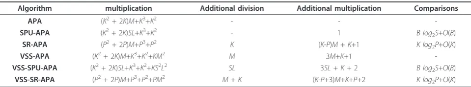
5. Computational complexity

The computational complexity of the VSS adaptive algorithms has been given in Tables 1 and 2. The com-putational complexity of the APA and NLMS is from [4]. The SPU-NLMS needs 3SL+1 multiplications. This algorithm needs 1 additional multiplication andB log2S +O(B) comparisons. Comparing the updated equation for NLMS and VSS-NLMS shows that the VSS-NLMS needs 4M + 3 additional multiplication and M division due to variable step-size. In VSS-SPU-NLMS, the addi-tional multiplication and addiaddi-tional division is respec-tively 4SL+ 3 and SL. Also, this algorithm needsB log2S +O(B) comparisons. It is obvious that the computational complexity of SPU-NLMS is lower than VSS-NLMS. The number of reductions in multiplication and division for VSS-SPU-NLMS is respectively 3(M-SL)-1 andM-SL.

The SPU-APA needs (K2+2K)SL+K3+K2multiplications. This algorithm needs 1 additional multiplication andB log2S+O(B) comparisons. The SR-APA needs (P2+2P)M +P3+P2multiplications andKdivisions. This algorithm needs (K-P)M+K+1 additional multiplications andK log2P +O(K) comparisons. Comparing the updated equation for APA and VSS-APA shows that the VSS-APA needs

Table 1 The computational complexity of NLMS, SPU-NLMS, VSS-NLMS, and VSS-SPU-NLMS algorithms

Algorithm multiplication Additional division Additional multiplication Comparisons

NLMS 3M+1 - -

-SPU-NLMS 3SL+1 - 1 B log2S+O(B)

VSS-NLMS 4M M 3M+4

-VSS-SPU-NLMS 4SL SL 3SL+5 B log2S+O(B)

Table 2 The computational complexity of APA, SPU-APA, SR-APA, VSS-APA, VSS-SPU-APA, and VSS-SR-APA

Algorithm multiplication Additional division Additional multiplication Comparisons

APA (K2_{+ 2K)M+K}3_+K2 _{- -}

-SPU-APA (K2_{+ 2K)SL+K}3_+K2 _{- 1 B log}

2S+O(B)

SR-APA (P2_{+ 2P)M+P}3_+P2 _{K (K-P)M+K+1 K log}

2P+O(K)

VSS-APA (K2_{+ 2K)M+K}3_+K2_+KM2 _{M 3M+K+1}

KM2+3M+K+1 additional multiplications andMdivisions due to variable step-size. In VSS-SPU-APA, the additional multiplication isKS2+L2+3SL+K+1 and additional division isSL. Also, this algorithm needsB log2S+O(B) compari-sons. It is obvious that the computational complexity of VSS-SPU-APA is lower than VSS-APA. The number of reductions in multiplication and division for VSS-SPU-APA is respectively (K2+2K+4)(M-SL)+K(M2-S2L2) and M-SL. In VSS-SR-APA, the additional multiplication is 3M+P+1 and additional division isMcompared with SR-APA. Also this algorithm needsK log2P+O(K) compari-sons. It is obvious that the computational complexity of VSS-SR-APA is lower than VSS-APA.

6. Experimental results

We presented several simulation results in system identification scenario. The unknown impulse response is generated according to hi = eiτ r(i), i = 0, ..., M-1, where r(i) is a white Gaussian random sequence with zero-mean and variance σ_r2 of 0.09 [20]. The length of impulse responses were set toM = 20, and 50 in simu-lations. Also, the envelope decay rateτwas set 0.04. The filter input is a zero-mean i.i.d. Gaussian process with variance σx2= 1. Another input signal is colored

Gaussian signal which is generated by filtering white Gaussian noise through a first-order autoregressive (AR (1)) system with the transfer function:

G(z)= 1

1−0.8Z−1 (88)

The white zero-mean Gaussian noise was added to the filter output such that the SNR = 15dB.

In all simulations, the MSD curves are obtained by ensemble averaging over 200 independent trials.

Figure 1 shows the MSD curves of APA, VSS-APA in [17], proposed VSS-APA, ES [19] and GNGD algorithm [16] for colored Gaussian input and M= 20. The para-meter Kwas set to 4 and different values for μ were used in APA. As we can see, by increasing the step-size, the convergence speed increases but the steady-state MSD also increases. The VSS-APA in [17] has both fast convergence speed and low steady-state MSD. The pro-posed VSS-APA has faster convergence speed and lower steady-state MSD than VSS-APA in [17], and classical APA.

In Figure 2 we presented the MSD curves for colored Gaussian input andM= 50. In this simulation, the para-meter Kwas set to 10. The results are also compared with APA with different values for the step-size and VSS-APA proposed in [17]. As we can see the perfor-mance of proposed VSS-APA has both fast convergence speed and low steady-state MSD features.

Figure 3 compares the MSD curves of SPU-APA, pro-posed VSS-APA, and propro-posed VSS-SPU-APA for colored Gaussian input and M= 20. The parametersK, and the number of blocks (B) were set to 4. In this fig-ure, the number of blocks to update (S) was set to 3 for SPU-APA. Again, different values for the step-size have been used in SPU-APA. The first one is (S/B), which is upper stability bound of SPU-APA, and the second one

0 1000 2000 3000 4000 5000 6000 7000 8000

-40 -30 -20 -10 0 10 20

Iteration Number

MS

D

in

d

B

(a) APA, _P=1 (b) APA, P=0.05

(c) VSS-APA proposed in [17] (d) Proposed-VSS-APA (e) GNGD, _P0= 0.2, _U=0.15 [16]

(f) ES [19]

(a) (b) (c) Input : Colored Gaussian signal

M=20, K=4

(e)

(f) _(d)

is (0.05 S/B) wich is low values for the step-size. As we can see, the convergence speed and steady-state MSD is changed by the step-size. The proposed VSS-SPU-APA has fast convergence speed and low steady-state MSD. The VSS-SPU-APA has been also compared with pro-posed VSS-APA. Close performance can be seen for these proposed algorithms. But the computational

complexity of proposed VSS-SPU-APA is lower than VSS-APA

Figure 4 presents the MSD curves of SPU-APA, pro-posed VSS-SPU-APA, and VSS-APA, for M = 50, and colored Gaussian input. The parameterKand the num-ber of blocks were set to 10, and 5 respectively. In this figure the parameterSwas set to 3, and different values

0 1000 2000 3000 4000 5000 6000 7000 8000

-40 -30 -20 -10 0 10 20 30 40 50

Iteration Number

MS

D

in

d

B

(a) APA, P=1

(b) APA, P=0.05

(c) VSS-APA proposed in [17] (d) Proposed-VSS-APA

(e) GNGD, P₀=0.5, U=0.15 [16]

(f) ES [19]

(a) (b) (c) (e)

(f) (d)

Input : Colored Gaussian signal M=50,K=10

Figure 2Comparing the MSD curves of APA with high and low step-sizes, variable step-size proposed in[17],proposed VSS-APA, GNGD[16]and ES[19]algorithms with M = 50, K = 10 and colored Gaussian signal as input.

0 1000 2000 3000 4000 5000 6000 7000 8000

-40 -30 -20 -10 0 10 20

Iteration Number

MS

D

in

d

B

(a) SPU-APA, B=4, S=3, P=S/B (b) SPU-APA, B=4, S=3, P=0.05S/B (c) Proposed-VSS-APA

(d) Proposed-SPU-APA, B=4, S=3

(a) (b) (c) (d) Input : Colored Gaussian signal

M=20,K=4

for the step-size have been used in SPU-APA. The simulation results show that the VSS-SPU-APA has good performance compared with SPU-APA. Also, the proposed VSS-APA, and VSS-SPU-APA have close per-formance. But the computational complexity of VSS-SPU-APA is lower than VSS-APA.

Figure 5 compares the MSD curves of SPU-NLMS, VSS-NLMS in [21], proposed VSS-SPU-VSS-NLMS, ES [19] and

GNGD algorithms [16]. The parametersB, andSwere set to 4, and 2 respectively. Various values for the step-size have been used for SPU-NLMS. The simulation results show that the proposed VSS-SPU-NLMS has fast conver-gence speed and low steady-state MSD features. Also this algorithm has close performance to VSS-NLMS in [21]. Good performance can be seen for proposed VSS-SPU-NLMS. This fact can be seen in Figure 6 forM= 50.

0 1000 2000 3000 4000 5000 6000 7000 8000

-40 -30 -20 -10 0 10 20 30 40

Iteration Number

MS

D

in

d

B

(a) SPU-APA, B=5, S=3, P=0.25S/B

(b) SPU-APA, B=5, S=3, P=0.0125S/B

(c) Proposed-VSS-APA

(d) Proposed-VSS-SPU-APA, B=5, S=3

(a) (b) (c) (d) Input : Colored Gaussian signal

M=50,K=10

Figure 4Comparing the MSD curves of SPU-APA with high and low step-sizes, proposed VSS-APA and proposed VSS-SPU-APA with M = 50, K = 10 and colored Gaussian signal as input.

0 1000 2000 3000 4000 5000 6000 7000 8000

-40 -30 -20 -10 0 10 20

Iteration Number

MS

D

in

d

B

(a) SPU-NLMS, B=4, S=2, P=2S/B (b) SPU-NLMS, B=4, S=2, P=0.2S/B (c) VSS-NLMS proposed in [21] (d) Proposed-VSS-SPU-NLMS (e) GNGD, P₀=.2, U=0.15 [16] (f) VSS-NLMS proposed in [17] (g) ES [19]

(c) (d)

(e) (a)

Input : Colored Ggaussian signal M=20

(f)

(g) (b)

Figure 7 compares the MSD curves of SR-APA, pro-posed VSS-SR-APA, and VSS-APA for colored Gaussian input signal. The parameter K was set 4. Again, large and small values for step-size have been used in SR-APA. As we can see, the proposed VSS-SR-APA has good convergence speed and low steady-state MSD. This figure shows that the proposed VSS-APA has bet-ter performance than proposed VSS-SR-APA. In Figure

8, we presented the results for M = 50, and colored Gaussian input signal. Comparing the MSD curves show that the VSS-SR-APA has also good performance in this case.

Figure 9 compares the MSD curves of proposed VSS-SPU-APA with S = 2 and S = 3, proposed-VSS-APA, ES [19], GNGD algorithm [16] and VSS-APA proposed in [17] with M = 20, K = 4 for colored

0 1000 2000 3000 4000 5000 6000 7000 8000

-35 -30 -25 -20 -15 -10 -5 0 5 10 15

Iteration Number

MS

D

in

d

B

(a) SPU-NLMS, B=5, S=3, P=1.5S/B (b) SPU-NLMS, B=5, S=3, P=0.5S/B (c) VSS-NLMS proposed in [21] (d) Proposed-VSS-SPU-NLMS (e) GNGD, _P0=0.3, rho=0.15 [16]

(f) VSS-NLMS, proposed in [17] (g) ES [19]

(a) (b) (c) (d) (e) (f) Input : Colored Gaussian signal

M=50

(g)

Figure 6Comparing the MSD curves of SPU-NLMS with high and low step-sizes, VSS-NLMS proposed in[17],VSS-NLMS proposed in [21],proposed VSS-SPU-NLMS, GNGD[16]and ES[19]algorithms with M = 50 and colored Gaussian signal as input.

0 1000 2000 3000 4000 5000 6000 7000 8000

-40 -30 -20 -10 0 10 20 30

Iteration Number

MS

D

in

d

B

(a) SR-APA, P=2, P=1

(b) SR-APA, P=2, P=0.05

(c) Proposed-VSS-APA (d) Proposed-VSS-SR-APA

(b) (c)

(d) (a)

Input : Colored Gaussian signal

M=20, K=4

Gaussian signal input. The simulation results show that the proposed VSS-APA has better performance than proposed VSS-APA in [17]. Also the perfor-mance of proposed VSS-SPU-APA for S = 3 is close to proposed VSS-APA.

Figure 10 compares the MSD curves of proposed VSS-SPU-NLMS with S = 1 andS = 2 andS = 3, proposed NLMS, ES [19], GNGD algorithm [16], and

VSS-NLMS proposed in [17] withM = 20,K= 4 for colored Gaussian signal input. This figure shows that the proposed VSS-NLMS has better performance than VSS-NLMS in [17]. Also by increasing the parameterS, the MSD curves of VSS-SPU-NLMS will be closed to VSS-NLMS.

Figure 11 presents the MSD curves of proposed VSS-SR-APA with P = 1 and P = 2 and P = 3 and

0 1000 2000 3000 4000 5000 6000 7000 8000

-40 -30 -20 -10 0 10 20 30 40

Iteration Number

MS

D

in

d

B

(a) SR-APA, P=3, P=1

(b) SR-APA, P=3, P=0.05

(c) Proposed-VSS-APA (d) Proposed-VSS-SR-APA

(d) (c) (b) (a) Input : Colored Gaussian signal

M=50, K=5

Figure 8Comparing the MSD curves of SR-APA with high and low step-sizes, proposed VSS-APA and proposed VSS-SR-APA with M = 50, K = 5 and colored Gaussian signal as input.

0 1000 2000 3000 4000 5000 6000 7000 8000

-40 -30 -20 -10 0 10 20

Iteration Number

MS

D

in

d

B

(a) VSS-APA proposed in [17] (b) Proposed-VSS-SPU-APA, B=4, S=2 (c) Proposed-VSS-SPU-APA, B=4, S=3 (d) Proposed-VSS-APA

(e) GNGD, P₀=0.2, U=0.15 [16]

(f) ES [21] Input : colored Gaussian signal

M=20, K=4

(a) (b) (c) (e)

(f) (d)

proposed VSS-APA, ES [19], GNGD algorithm [16], and VSS-APA proposed in [17] with M = 20, K = 4 for colored Gaussian signal input. This figure shows that the performance of SR-APA is better than VSS-APA in [17]. Also, by increasing the parameterP, the performance of SR-APA will be closed to VSS-APA.

Finally, we justified the tracking performance of the proposed methods in Figure 12. The impulse response variations are simulated by toggling between different impulse responses hi = e-iτ r(i) and gi = eiτ r(i). The impulse response is changed to gi =eiτ r(i) at iteration 4000. As we can see, the proposed VSS algorithms have good tracking performance. The proposed VSS-APA has

0 1000 2000 3000 4000 5000 6000 7000 8000

-35 -30 -25 -20 -15 -10 -5 0 5 10 15

Iteration Number

MS

D

in

d

B

(a) VSS-NLMS proposed in [17] (b) Proposed-VSS-SPU-NLMS, B=4, S=1 (c) Proposed-VSS-SPU-NLMS, B=4, S=2 (d) Proposed-VSS-SPU-NLMS, B=4, S=3 (e) Proposed-VSS-NLMS

(f) GNGD, P₀=0.2, U=0.15 [16] (g) ES [19]

(a) (b) (c) (e)

(g) (f)

(d) Input : colored Gaussian signal

M=20, K=4

Figure 10Comparing the MSD curves of proposed VSS-SPU-NLMS with S = 1 and S = 2 and S = 3, proposed VSS-NLMS, VSS-NLMS proposed in[17],GNGD[16]and ES[19]algorithms with M = 20, K = 4 and colored Gaussian signal as input.

0 1000 2000 3000 4000 5000 6000 7000 8000

-40 -30 -20 -10 0 10 20

Iteration Number

MS

D

in

d

B

(a) VSS-APA proposed in [17] (b) Proposed-VSS-SR-APA, P=1 (c) Proposed-VSS-SR-APA, P=2 (d) Proposed-VSS-SR-APA, P=3 (e) Proposed-VSS-APA (f) GNGD, P0=0.2, U=0.15 [16] (g) ES [19]

Input : colored Gaussian signal M=20, K=4

(a) (b) (c) (d)

(e) (f) (g)

better performance than other algorithms. The perfor-mance of proposed VSS-SPU-APA with B= 4, andS= 3 is close to proposed VSS-APA.

7. Conclusions

In this paper, we presented the novel VSS adaptive fil-ter algorithms such as VSS-SPU-NLMS, VSS-APA, VSS-SR-APA and VSS-SPU-APA based on prior knowledge of the channel impulse response statistic. These algorithms exhibit fast convergence while redu-cing the steady-state MSD as compared to the ordinary SPU-NLMS, APA, SR-APA and SPU-APA algorithms. The presented algorithms were also computationally efficient. We demonstrated the good performance of the presented VSS adaptive algorithms in system iden-tification scenario.

Received: 2 December 2010 Accepted: 8 November 2011 Published: 8 November 2011

References

1. B Widrow, SD Stearns, Adaptive Signal Processing (Englewood Cliffs, NJ: Prentice-Hall, 1985)

2. S Haykin,Adaptive Filter Theory, 4th edn. (NJ: Prentice-Hall, 2002) 3. K Ozeki, T Umeda, An adaptive filtering algorithm using an orthogonal

projection to an affine subspace and its properties, inElectron Commun Jpn. 67-A, 19_–27 (1984)

4. AH Sayed,Fundamentals of Adaptive Filtering(Wiley, 2003)

5. S Roy, JJ Shynk, Analysis of data-reusing LMS algorithm, inProc Midwest Symp Circuits Syst, 1127–1130 (1989)

6. HC Shin, WJ Song, AH Sayed, Mean-square performance of data-reusing adaptive algorithms. IEEE Signal Processing Letters12(12), 851–854 (Dec 2005)

7. SS Pradhan, VE Reddy, A new approach to sub band adaptive filtering. IEEE Trans Signal Processing47, 655–664 (1999). doi:10.1109/78.747773

8. KA Lee, WS Gan, Improving convergence of the NLMS algorithm using constrained sub band updates. IEEE Signal Processing Letters11(9), 736–739 (2004). doi:10.1109/LSP.2004.833445

9. OW Kwong, ED Johnston, A variable step-size LMS algorithm. IEEE Trans Signal Processing40(7), 1633–1642 (1992). doi:10.1109/78.143435 10. T Aboulnasr, K Mayyas, A robust variable step-size lms-type algorithm:

Analysis and simulations. IEEE Trans Signal Processing45(3), 631–639 (1997). doi:10.1109/78.558478

11. DI Pazaitis, AG Constantinides, A novel kurtosis driven va riable step-size adaptive algorithm. IEEE Trans Signal Processing47(3), 864–872 (1999). doi:10.1109/78.747793

12. VJ Mathews, Z Xie, A stochastic gradient adaptive filter with gradient adaptive step size. IEEE Trans Signal Processing41(6), 2075_–2087 (1993). doi:10.1109/78.218137

13. V Krishnamurthy, Averaged stochastic gradient algorithms for adaptive blind multiuser detection in DS/CDMA systems. IEEE Trans Communications 48(1), 125–134 (2000). doi:10.1109/26.818880

14. RC de Lamare, R Sampaio-Neto, Low-complexity blind variable step size mechanisms for minimum variance CDMA receivers. IEEE Transactions on Signal Processing54(6), 2302_–2317 (2006)

15. Y Cai, RC de Lamare, Low-Complexity Variable Step Size Mechanism for Code-Constrained Constant Modulus Stochastic Gradient Algorithms applied to CDMA Interference Suppression. IEEE Transactions on Signal Processing57(1), 313_–323 (2009)

16. DP Mandic, A Generalized Normalized Gradient Descent Algorithm. IEEE Signal Processing Letters11(2), 115–118 (2004). doi:10.1109/

LSP.2003.821649

17. HC Shin, AH Sayed, WJ Song, Variable step-size NLMS and affine projection algorithms. IEEE Signal Processing Letters11(2), 132_–135 (Feb 2004). doi:10.1109/LSP.2003.821722

18. MSE Abadi, V Mehrdad, A Gholipour, Family of Variable Step-Size Affine Projection Adaptive Filtering Algorithms with Selective Regressors and Selective Partial Update. International Journal of Science and Technology, Scientia, Iranica17(1), 81–98 (2010)

19. S Makino, Y Kaneda, N Koizumi, Exponentially weighted step-size NLMS adaptive filter based on the statistics of a room impulse response. IEEE Transactions on Speech Audio Processing1(1), 101–108 (1993). doi:10.1109/ 89.221372

20. N Li, Y Zhang, Y Hao, JA Chambers, A new variable step-size NLMS algorithm designed for applications with exponential decay impulse responses. Signal Processing88(9), 2346–2349 (2008). doi:10.1016/j. sigpro.2008.03.002

0 1000 2000 3000 4000 5000 6000 7000 8000

-40 -30 -20 -10 0 10 20 30

Iteration Number

MS

D

in

d

B

(a) Proposed-VSS-SPU-NLMS, B=4, S=3 (b) VSS-APA proposed in [17]

(c) Proposed-VSS-SR-APA, P=2 (d) Proposed-VSS-SPU-APA, B=4, S=3 (e) Proposed-VSS-APA

(b)

(c) (d)

(e)

(a) Input : white Gaussian signal

M=20, K=4

21. Kun Shi, Xiaoli Ma, A variable-step-size NLMS algorithm using statistics of channel response. Signal Processing90(6), 2107_–2111 (2010). doi:10.1016/j. sigpro.2010.01.015

22. SC Douglas, Analysis and implementation of the max-NLMS adaptive filter, inProc 29th Asilomar Conf on Signals, Systems, and Computers, Pacific Grove, CA, 659_–663 (1995)

23. T Schertler, Selective block update NLMS type algorithms, inProc IEEE Int Conf on Acoustics, Speech, and Signal Processing,Seattle, WA, 1717_–1720 (1998)

24. K Dogancay, O Tanrikulu, Adaptive filtering algorithms with selective partial updates. IEEE Trans Circuits, Syst. II: Analog and Digital Signal Processing 48(8), 762–769 (2001). doi:10.1109/82.959866

25. MSE Abadi, JH Husøy, Mean-square performance of adaptive filters with selective partial update. Signal Processing88(8), 2008–2018 (2008). doi:10.1016/j.sigpro.2008.02.005

26. K Dogancay, Partial-Update Adaptive Signal Processing: Design, Analysis and Implementation, (Academic Press, 2008)

27. KY Hwang, WJ Song, An affine projection adaptive filtering algorithm with selective regressors. IEEE Trans Circuits, Syst. II: EXPRESS BRIEFS54, 43–46 (2007)

28. MSE Abadi, H Palangi, Mean-square performance analysis of the family of selective partial update and selective regressor affine projection algorithms. Signal Processing90(1), 197–206 (2010). doi:10.1016/j.sigpro.2009.06.013

doi:10.1186/1687-6180-2011-97

Cite this article as:Shams Esfand Abadi and AbbasZadeh Arani:A family of variable step-size affine projection adaptive filter algorithms using statistics of channel impulse response.EURASIP Journal on Advances in Signal Processing20112011:97.

Submit your manuscript to a

journal and benefi t from:

7Convenient online submission

7Rigorous peer review

7Immediate publication on acceptance

7Open access: articles freely available online

7High visibility within the fi eld

7Retaining the copyright to your article