OF DAMAGE BY VOID NUCLEATION AND
GROWTH
Thesis by
Celia Reina Romo
In Partial Fulfillment of the Requirements for the Degree of
Doctor of Philosophy
California Institute of Technology Pasadena, California
2011
c
2011
Acknowledgements
I owe so much to so many people, that this acknowledgment section cannot be complete. I will therefore explicitly thank a few people and hope to implicitly thank the rest of them. First and foremost I truly want to thank my supervisor Professor Michael Ortiz. It has been a great honor to work with him as well as an extremely fun experience. The work written here is the result of many hours of exciting discussions and it would not have been possible without his guidance, his enthusiasm and his continuous encouragements and efforts towards our objectives. ¡Gracias Miguel!. The second person to whom I am very grateful is Jaime Marian. I had the pleasure to work with him during a 10-week stay at Lawrence Livermore National Laboratory and since then, he has served as a mentor and a friend. Chapter2 is work that has been done in very close collaboration with him. I would like to thank my committee members, Professor Guruswami Ravichandran, Professor Kaushik Bhattacharya and Professor Chiara Daraio, for their expert advice on my thesis work as well as on my future plans. I would like to acknowledge as well the support received from the faculty members at my university in Seville. In particular, I would like to thank Pilar Ariza who made possible my arrival at Caltech through the Fellowship from the Agency of Innovation and Development of Andalusia. Very certainly, this thesis would have not happened without it.
I also owe my deepest gratitude to Paco, who has always been available for discussion and has shown his support in many different ways, and to my colleagues and friends Luigi, Olive, Sigrid, Kerstin, Phanish, Daniel and Malena amongst others. Interaction with them was highly beneficial for the completion of this work. In addition, I would like to give special thanks to Bo, who made possible the parallel simulations shown in Section
3.8.
during all these years.
Abstract
Voids are observed to be generated under sufficient loading in many materials, ranging from polymers and metals to biological tissues. The presence of these voids can have drastic implications at the macroscopic level including strong material softening and more incipient fracture. Developing tools to appropriately account for these effects is therefore very desirable.
This thesis is concerned with both, the appearance of voids (nucleation process) and the modeling and simulation of materials in the presence of voids. A particular nucle-ation mechanism based on vacancy aggregnucle-ation in high purity metallic single crystals is analyzed. A multiscale model is developed in order to obtain an approximate value of the time required for vacancies to form sufficiently large clusters for further growth by plastic deformation. It is based on quantum mechanical results, kinetic Monte Carlo methods and continuum mechanics estimates calibrated with quasi-continuum results. The ulti-mate goal of these simulations is to determine the feasibility of this nucleation mechanism under shock loading conditions, where the temperature and tensions are high and vacancy diffusion is promoted.
Contents
Acknowledgements iv
Abstract vi
Contents viii
List of Figures xi
List of Tables xvii
1 Introduction 1
2 Nucleation of voids 8
2.1 Introduction . . . 8
2.2 Physical model . . . 11
2.3 Kinetic Monte Carlo . . . 11
2.4 Rate catalog . . . 13
2.5 Clustering kinetics . . . 17
2.6 Application to spall fracture . . . 20
2.6.1 Critical pressure for plasticity induced void growth . . . 25
2.6.1.1 Pressure induced by the surface energy . . . 26
2.7 Notes on the numerical implementation of the serial code . . . 27
3 Material response under void damage 34 3.1 Previous micromechanical models of void growth. . . 36
3.1.1 Strain hardening and kinematic hardening . . . 40
3.1.3 Void shape anisotropy . . . 41
3.1.4 Plastic anisotropy . . . 42
3.1.5 Influence of shear on damage evolution . . . 42
3.1.6 Inertia effects . . . 43
3.2 Micromechanical model for void growth . . . 45
3.3 Effective constitutive behavior . . . 49
3.3.1 Static case without body forces . . . 52
3.3.2 Static case with body forces . . . 54
3.3.3 Dynamic case without separation of time scales . . . 56
3.3.4 Dynamic case with separation of time and length scales . . . 61
3.3.4.1 The spacetime formulation of nonlinear elastodynamics . . 61
3.3.4.2 Spacetime averaging . . . 65
3.4 Time discretization . . . 71
3.4.1 Implicit dynamics . . . 72
3.4.2 Explicit dynamics . . . 75
3.5 Spatial discretization of the hollow sphere . . . 77
3.5.1 Boundary conditions . . . 80
3.5.2 Quadrature rule . . . 81
3.5.3 Elastic moduli . . . 82
3.6 Verification . . . 84
3.6.1 Static volumetric deformation of a porous Hookean material . . . . 84
3.6.1.1 Analytic solution . . . 84
3.6.1.2 Convergence analysis . . . 85
3.6.2 Static axisymmetric deformation of a porous Hookean material . . . 86
3.6.2.1 Analytic solution . . . 86
3.6.2.2 Convergence analysis . . . 88
3.6.3 Static volumetric deformation of a porous neo-Hookean material . . 88
3.6.3.1 Analytic solution . . . 89
3.6.3.2 Convergence analysis . . . 90
3.6.4 Static arbitrary deformation of a porous neo-Hookean material . . . 91
3.6.6 Dynamic volumetric deformation of a porous neo-Hookean material.
Explicit dynamics formulation. . . 92
3.7 Material point calculations . . . 95
3.7.1 Static . . . 95
3.7.1.1 Elastic material . . . 95
3.7.1.2 Plastic material . . . 97
3.7.2 Dynamic . . . 103
3.7.2.1 Explicit dynamics . . . 103
3.8 Numerical example . . . 105
3.8.1 Experiments . . . 105
3.8.2 Material modeling without porosity . . . 107
3.8.2.1 Hyperelastic model at low strain rates . . . 107
3.8.2.2 Viscoelastic model for polyurea . . . 109
3.8.2.3 Complete model for polyurea . . . 118
3.8.3 Material modeling with porosity . . . 118
3.8.4 Comparison with experiments . . . 118
4 Concluding remarks and further directions 123 A Exact integration of the stiffness matrix 126 B Exact integration of the mass matrix 137 C Void volume fraction 139 C.1 Exact integration . . . 140
D Viscoelastic parameters in a relaxation test. Incompressible case 142 E Non-constant value of the Poisson’s ratio for a compressible viscoelastic material 144 F Exact viscoelastic parameters for a compressible material 146 F.0.1 Exact relaxation curve with one term of the Prony series . . . 148
List of Figures
1.1 Presence of voids in different materials. (a) Plastically deformed zone
sur-rounding an incipient void. Belak (2005). (b) Scanning electron micro-graph of the fracture surface of rubber-modified epoxy polymers. Azimi et al. (1996). (c) Quasi-static rupture of a copper sample. Curran et al.
(1977). (d) Experimental observation of kidney tissue subjected to shock-wave lithotripsy. Bailey et al.(2003). (e) Partial spall on a 5 mm aluminum plate of commercial purity. Curran et al. (1977). . . 2
1.2 Various nucleation sites. (a) Void growth within an inclusion colony in a
low-alloy, quenched and tempered steel. Hancock and Mackenzie (1976). (b) Nucleation of spherical voids at grain boundary and grain boundary
triple point. Christy et al. (1986).. . . 5
2.1 Frequency line (aggregate of the individual rates) and schematic
represen-tation of the procedure for selecting a vacancy movement with probability
pi = Rrmaxi . . . 12 2.2 Schematic representation of the null events in the synchronous parallel
Ki-netic Monte Carlo proposed byMartinez et al. (2008) . . . 13
2.3 Speed improvement obtained with the parallel implementation as a function
of the number of processors K. Both codes ran on 2.4GHz processors with 16GB of memory per node. Version 1 MPI was used for the parallel
imple-mentation. The system analyzed consists of 105 vacancies atT = 728 K and εvv = 0. . . 14 2.4 Schematic representation of the movement of a vacancy (red color) to a
neighboring position with a higher energy (left figure) or lower energy (right
2.5 QC-OFDFT calculations for aluminum (Gavini,2008). (a) Di-vacancy bind-ing energies versus macroscopic volumetric strain. (b) Migration energy
ver-sus macroscopic volumetric strain. . . 16
2.6 OFDFT calculations for aluminum (Ho et al., 2007). Jump frequency as a function of the volumetric deformation. . . 16
2.7 118 nm cubic periodic cell of fcc aluminum (∼108atoms) containing at 0.1%
concentration (∼105 vacancies),T = 728 K, and εvv= 0. . . 17 2.8 118 nm cubic periodic cell of fcc aluminum (∼ 108 atoms) containing at
0.1% concentration (∼105 vacancies),T = 728 K, andεvv= 0. Evolution of histogram of cluster sizes. . . 18
2.9 100,000 vacancies at concentration of 0.1% (108 atoms). Influence of
volu-metric strain and temperature. . . 19
2.10 100,000 vacancies. T= 728K, εvv= 0. . . 19 2.11 Equilibrium concentration of vacancies versus volumetric strain at different
temperatures. . . 21
2.12 (a) Heat capacity at constant pressure versus temperature. (b) 0 K equation
of state extended to positive temperatures through a Mie-Gr¨uneisen equation
of state. . . 23
2.13 Critical cluster size in aluminum as a function of volumetric strain and
tem-perature. The corresponding pressures at the different temperatures are
indicated on the right ordinate axis. . . 24
2.14 Time required for the formation of critical nanovoids capable of growing by
dislocation-mediated plasticity as a function of the volumetric deformation
and temperature. Solid lines represent tanh fits of the data. . . 24
3.1 Yield function as a function of the hydrostatic stress for several values of the
void volume fraction. (Tvergaard, 1982) . . . 38
3.2 Space filling construction. . . 46
3.3 Deformation of the representative volume element according to the
macro-scopic deformation mappingϕM and the macroscopic deformation gradient
3.4 Boundary value problem over a hollow sphere of inner radius a and outer radius b. . . 48
3.5 Representative spacetime domain at the macroscopic and microscopic level.. 66
3.6 Examples of deformed shapes that can be obtained through a spherical
har-monic expansion of the displacement field until degreel. . . 79
3.7 Number of degrees of freedom of the finite element formulation of the hollow
sphere as a function of the number of layers in the radial direction and the
order of the expansion in spherical harmonics. . . 79
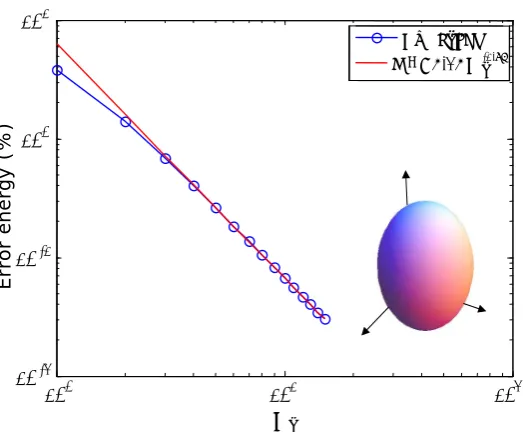
3.8 Error in the energy as a function of the number of elements in the radial
direction. Parametersa= 1, b= 2, λ= 1, µ= 1, Nl= 1, ε11=ε22 =ε33 = 0.05 86
3.9 Error in the energy as a function of the number of elements in the radial
direction. Parameters a = 1, b = 2, λ = 1, µ = 1, Nl = 3, ε11 = ε22 =
0.05, ε33= 0.1. . . 89
3.10 Error in the energy as a function of the number of elements in the radial
direction. Parametersa = 1, b = 2, λ= 1, µ = 1, Nl = 1, F11 =F22 =F33 =
1.2. . . 90
3.11 Error in the energy as a function of the number of elements in the radial
direction. Parameters a = 1, b = 2, λ = 1, µ = 1, Nl = 5, F11 = 1.2, F12 =
0.1, F13 = 0.18, F21 = 0.2, F22 = 1.1, F23 = 0.21, F31 = 0.15, F32 = 0.3, F33 =
1.15. . . 91
3.12 Error in the energy as a function of the number of elements in the radial
direction. Parameters a = 1, b = 2, Nl = 3. Uniaxial deformation, F11 =
1.2, F22 = 1.0, F33 = 1.0. . . 92
3.13 Stress-strain curve for a porous neo-Hookean material (Table 3.1) subjected
to volumetric deformation. Comparison of two mesh sizes and two time steps. 93
3.14 Error in the energy as a function of the number of elements in the radial
direction. Spherical expansion,F11=F22=F33 = 1.1. . . 93
3.15 Material response under spherical expansion at constant strain rate.
3.16 Volumetric expansion response for different void volume fractions. The
nu-merical solutions are obtained with Nr = 10 and Nl = 1. (a) Evolution of the pressure. (b) Evolution of the void volume fraction.. . . 96
3.17 Response for different void volume fractions and different loading conditions.
The numerical solutions are obtained withNr = 10 andNl = 1. (a) Uniaxial strain response. (b) Evolution of the void volume fraction under uniaxial
strain. (c) Uniaxial stress response. (d) Evolution of the void volume fraction
under uniaxial stress. (e) Simple shear response. (f) Evolution of the void
volume fraction under simple shear.. . . 98
3.18 Volumetric expansion response for different void volume fractions. The
nu-merical solutions are obtained with Nr = 10 and Nl = 1. (a) Evolution of the pressure. (b) Evolution of the void volume fraction.. . . 99
3.19 Response for different void volume fractions and different loading conditions.
(a) Uniaxial strain response. (b) Evolution of the void volume fraction under
uniaxial strain. (c) Uniaxial stress response. (d) Evolution of the void
vol-ume fraction under uniaxial stress. (e) Simple shear response. (f) Evolution
of the void volume fraction under simple shear. . . 100
3.20 Initial yield of the representative volume element with zero and finite void
volume fraction, compared to Gurson’s yield surface. Parameters a= 1, b= 2, Nr = 10, Nl = 1. The red diamond on the x-axis indicates the analytical solution for initial yield of a rigid perfectly plastic hollow sphere. . . 101
3.21 Gurson’s model (continuous lines) versus numerical predictions (discrete
symbols) of complete yield of the hollow sphere. Stress measures normalized
with respect to the minimum (‘x’ symbols) and the maximum (‘o’ symbols)
microscopic yield stress attained in the domain. . . 102
3.22 Evolution of a hollow sphere of 12.5% void volume fraction under uniaxial
strain. . . 102
3.23 Material response under spherical expansion at constant ¨εwith varying den-sity. Comparison to static solution. . . 103
3.24 Taylor anvil test of polyurea rod. Experiments performed by Mock et al. at
3.25 Post impact images of the polyurea rod. Experiments performed by Mock
et al. at NSWC. (a)v = 245 m/s. (b) v = 332 m/s. . . 106
3.26 Fit of the quasi-static behavior of the polyurea ( ˙ε = 0.0016 s−1) with differ-ent hyperelastic material models. . . 109
3.27 Uniaxial compression stress-strain behavior of polyurea at several true strain
rates (Sarva et al., 2007). . . 110
3.28 Master curve resulting from normalizing the experimental stress-strain
rela-tion of Sarva et al. (2007). . . 112
3.29 Evolution of the true strain rate in the uniaxial compression experiments
performed by Sarva et al. (2007). . . 113
3.30 Comparison of the developed material model and the experimental results
of Sarva et al. (2007) at different strain rates. . . 113
3.31 Comparison of the master curve obtained with the developed material model
and the experimental results of Sarva et al. (2007) at different strain rates. . 114
3.32 Strain history obtained from the experimental true strain rate versus true
strain history and fit to the curve with a quadratic polynomial. (a) ˙ε = 6500s−1. (b) ˙ε= 9000s−1. . . 116
3.33 Comparison of the stress-strain response of the material model and the
ex-periments performed by Sarva et al. (2007) at several strain rates. . . 117
3.34 Verification of the constant strain rate assumption. . . 117
3.35 Comparison of the uniaxial material response between experiments (Sarva et al., 2007), non-porous material model, and porous material model with two void volume fractions. . . 119
3.36 Fine mesh ( 48000 nodes and 20000 elements) and coarse mesh ( 6000 nodes
and 2500 elements) used in the finite element simulation of the Taylor test. 120
3.37 Comparison between experiments (Mock et al.)and simulations with two different mesh sizes. (a) Evolution of the normalized length versus time. (b)
Evolution of the normalized radius versus time. . . 121
3.39 Numerical evolution of the Taylor bar experiment at v = 332 m/s with the porous material model at initial porosity of 1.5 %.. . . 122
3.40 Void volume fraction distribution at 32 µs. . . 122
List of Tables
3.1 Material properties of the porous neo-Hookean material. . . 93
3.2 Material properties of a typical alluminum alloy.. . . 104
3.3 Material properties of the porous neo-Hookean material. . . 104
3.4 Fitting parameters of the Ogden model. . . 108
Chapter 1
Introduction
Voids are observed to be generated under sufficient loading in many materials (see 1.1), ranging from polymers (Gent and Lindley,1958, Huang and Kinloch, 1992, Azimi et al.,
1996) and metals (Tvergaard,1990) to biological tissues (Pishchalnikov et al.,2003). Even materials that are nominally “pure” are seen to develop voids in order to accommodate the applied deformation (Bauer and Wilsdorf, 1973).
The presence of initial microscopic defects in the form of voids can have drastic impli-cations at the macroscopic level. In the case of elastomers, the maximum pressure that the solid can sustain changes from a theoretical infinite value for an undamaged material, to a well defined finite value when those defects are considered (Ball, 1982). This critical pressure is associated to a sudden increase in the void volume fraction, a phenomenon called cavitation, which weakens the material and ultimately leads to the fracture of the specimen. In the case of metals, small void volume concentrations can also substantially alter the plastic behavior. The usual assumption of plastic incompressibility does not hold from a macroscopic perspective in the presence of voids. An effective change in volume occurs by void growth and incompressible plastic deformation of the matrix surround-ing the cavity. As a result, both, the yield surface of the porous material and fracture initiation, become sensitive to volumetric stress states (Hancock and Mackenzie, 1976,
(a) (b)
(c) (d)
(e)
to a particular nucleation mechanism of interest in ductile failure. It is based on vacancy diffusion in high-purity metallic single crystals under extreme conditions. Damage evolu-tion under preexistent voids, on the other hand, is treated within the general framework of continuum mechanics and is therefore applicable to any material.
Throughout this thesis a multiscale approach is adopted so as to root the behavior of the material at a given scale in the response at the lower scales. In the classical de-scription of materials, the effective response is characterized by a few numbers, called “material parameters”, which allow us to describe the behavior in a simplistic way, hiding the underlying complexity that is ultimately responsible for such behavior. This includes parameters such as Young’s modulus, Poisson’s ratio, strain hardening or critical energy release rate at the macroscopic level, and diffusion coefficient or cohesive energy for in-stance, at an atomistic level. This simplification is very appealing. The problem relies on the fact that these “material properties” are not really intrinsic. Rather, they can be highly dependent on the load history of the material in question, and a single set of numbers is unable to describe the response under varying conditions. This is particularly true in the presence of damage, which is the situation of interest in the present study. The ultimate goal of this type of multiscale models is to enable numerical simulations with pre-dictive capability. This would be very desirable as a design tool, reducing tremendously the experimental costs, and would also allow us to be predictive in situations where ex-periments are not possible. Current limitations of multiscale models lie in validation at the lower scales, which is of great experimental difficulty. However, recent experimental developments, such as X-ray tomography (Maire et al., 2005, Morgeneyer et al., 2008) or high-angle annular dark-field imaging in a scanning transmission electron microscopy (Voyles et al.,2002,Kaiser et al.,2002) hold great promise for generating accurate models. Ductile failure, which is of high interest in industrial applications and in this work, is an example of a complex process that is inherently multiscale. More particularly, this type of failure occurs via nucleation, growth, and coalescence of voids (Garrison and Moody,
as previously mentioned, such critical values are not really material parameters. This is especially the case for ductile materials, in which the the crack advance is governed by the nucleation and growth of voids, a phenomenon that is dependent on the com-plete load history (Curran et al.,1977). This observation has lead to the development of more physically based descriptions of fracture (see review paper Pineau (2006)). Due to its importance, a large number of authors have contributed to the field with more phe-nomenological continuum damage mechanic theories (Tuler and Butcher,1968,Chaboche,
1988), micromechanically based models (Gurson, 1977a, Curran et al., 1977, Koplik and Needleman,1988,Tvergaard,1990,Pardoen and Hutchinson,2000,Rudd and Broughton,
2000,Antoun et al.,2003, Weinberg and Ortiz, 2009) or molecular dynamics simulations (Rudd and Belak,2002,Sepp¨al¨a et al.,2004,Marian et al., 2004, 2005, Ahn et al., 2007,
Potirniche et al., 2006, Zhu et al., 2007, Dvila et al., 2005). A complete review of the different proposed approaches is out of the scope of this manuscript. Only the relevant background for the work presented here is summarized in the corresponding chapters.
The goal of this thesis is to develop nucleation and growth models that could ultimately be included in a complete multiscale model of failure. These two phenomena are treated independently here. The rigorous connection between them and the study of the final stage of failure remains an open problem that requires further analysis. In the following, a brief introduction to the nucleation in ductile materials is presented and an outline of the work developed in each chapter is provided.
It is well known that void nucleation in ductile materials occurs mainly at second-phase particles by interfacial decohesion or particle fracture (Puttick, 1959, Goods and Brown,
1979). See for instance, Fig.1.2(a), where the growth of voids within an inclusion colony is shown. Models for this type of nucleation exist and are usually based on the stresses or the strains at the interface (Gurson, 1977b, Neddleman, 1987). In polycrystals, grain boundaries and triple points are also weak points that supply preferred nucleation sites (Hull and Rimmer, 1959, Christy et al., 1986, Belak, 1998, Rudd and Belak, 2002). Fig.
during plastic deformation, irradiation, quenching, or by other means (Cawthorne and Fulton, 1967). Chapter 2 addresses this latter mechanism. In particular, the attempt is to estimate critical times required for the nucleation of nanovoids via vacancy aggregation in high-purity single crystals and to determine if it is fast enough to operate under shock loading conditions.
(a) (b)
Figure 1.2: Various nucleation sites. (a) Void growth within an inclusion colony in a low-alloy, quenched and tempered steel. Hancock and Mackenzie (1976). (b) Nucleation of spherical voids at grain boundary and grain boundary triple point. Christy et al. (1986).
results at the lower scales. In particular, a kinetic Monte Carlo approach is used to describe the discrete atomic jumps. Such a model uses jump rates that emanate from statistical mechanics, and the parameters involved are taken from quantum mechanical calculations, in particular orbital-free density functional theory. Finally, this atomistic model is used to determine the time required for vacancies to aggregate into clusters of a size that is visible macroscopically under shock loading conditions. The proposed nucleation criterion is based on the critical size for subsequent growth by dislocation-mediated plasticity (seeMeyers et al.(2009) for a review of the role of dislocations on void growth). A continuum mechanics estimate calibrated with quasi-continuum models of void growth (Marian et al., 2004) is developed to determine such critical size. The computed nucleation times resulting from the analysis suggest that vacancy aggregation and cluster coarsening is a feasible mechanism of nanovoid nucleation in high-purity aluminum single crystals over pulse durations, temperatures and tensile volumetric strains typical of, for example, spall tests.
In Chapter 3, an attempt is made towards defining the overall dynamic behavior of materials where voids have already nucleated. This is done through a two-level repre-sentation of the material. The lower scale, termed “microscopic”, is treated through a representative volume element (RVE) composed of two phases: a homogeneous matrix and voids. The behavior of the RVE is then suitably averaged to provide the so called macroscopic behavior of the material, which is now treated as homogeneous. The connec-tion between the two scales is well understood for the static case under infinitesimal (Hill,
1963, 1967) and large strains (Hill, 1972, Ogden, 1974, Casta˜neda, 1991, Nemat-Nasser,
1999). However, the connection between the micro and macro levels is less well understood under dynamic loading, and little can be found in the literature in that respect (Molinari and Mercier,2001,Wang and Sun,2002). The work presented in the first part of Chapter
time. The formulation presented is not restricted to this particular case of heterogeneity. The range of applications is very wide and extends to composites and materials with evolving microstructure.
The second part of Chapter 3 is dedicated to the spatial discretization. The RVE chosen to represent porous materials is the hollow sphere, as thought of byGurson(1977a). A particular type of finite element, adapted to the considered geometry, is developed. It consists of an approximation space based on spherical harmonics. This set of functions constitutes a complete orthogonal space on the sphere, and is therefore suitable for a finite element discretization. Two specific properties make this discretization advantageous with respect to more standard finite element formulation. First, it allows a representation of the different fields on the sphere with a very low number of degrees of freedom, and secondly and most importantly, the symmetries of the porous material, if existent, are respected upon discretization. The necessary tools for solving boundary value problems on the hollow sphere are also provided. This includes a quadrature rule that integrates exactly the stiffness matrix, the mass matrix and the void volume fraction under the proposed discretization; and an explicit analytic formula for imposing the boundary conditions that emanated from the consistent two-level representation of the porous material.
The resulting finite element procedure has been verified extensively. Comparisons with several analytic solutions are performed and convergence analyses indicate close to ideal convergence rates for different materials under arbitrary loading conditions. This work is then concluded by the multiscale simulation of a real example problem in order to demonstrate its applicability. The example consists of a high speed Taylor test of polyurea material. A material model for polyurea is proposed and the results are compared with experimental observations.
Chapter 2
Nucleation of voids
2.1
Introduction
This chapter is concerned with the nucleation of voids via diffusion-mediated vacancy aggregation in high-purity metallic single crystals. This is an accepted nucleation mech-anism in failure under creep at elevated temperatures (Raj and Ashby, 1975, Cocks and Ashby, 1982). More debate exists, though, in the literature as to its viability as a nucle-ation mechanism in fast failure processes under extreme conditions. The present work is concerned with the latter. More precisely, a multiscale model based on first principles is developed. It allows the determination of the time required for the voids to attain a size that can alter the macroscopic behavior.
The details of these diffusion processes can be computed accurately by means of molec-ular dynamic calculations (Sinno et al., 1996, Hastings et al., 1997, Belak, 1998, Rudd and Belak, 2002), in which the classical equations of motion for the system of atoms are propagated in time. Such computations require the use of very small time steps in the numerical analyses (∼ 10−15) and resolve the atomic vibrations, which are not of interest in the present study. Another methodology widely used in diffusive processes is the kinetic Monte Carlo method (Young and Elcock, 1966, A. La Magna, 1999, Haley et al., 2006). In this approach, only the discrete jumps of the vacancies are considered, but an a priori knowledge of the microscopic motions and their rates is required. This is not always trivial, as demonstrated by examples found in the literature of complex non-intuitive transitions occurring in surface and bulk diffusion (Liu and Adams, 1992,
Uberuaga et al., 2004). Failure to consider some physically possible motions can lead to an erroneous evolution of the system. Within kinetic Monte Carlo (KMC), the rates of the motions are commonly obtained with transition state theory (Vineyard,1957), which borrows elements from statistical mechanics. A third alternative to describe the vacancy diffusion process relies on continuum descriptions (Seitz, 1948, Penrose, 1997, Weinberg and B¨ohme, 2009). The concentration of vacancies is thought of as a function of space and time, and evolution equations are used to describe its progression. This constitutes a more phenomenological description of the diffusion process, but allows the study of very large systems over a long period of time.
As a compromise between accuracy and size of the domain and time span that can be explored computationally, a lattice kinetic Monte Carlo (LKMC) approach is used in this work. A brief review of the algorithms used in the simulations (Bortz et al., 1975,
Martinez et al., 2008) is presented in Section 2.3. The required rates of the possible motions are computed by transition state theory with parameters obtained from Orbital Free Density Functional Theory (OFDFT) calculations (Gavini, 2009a, Ho et al., 2007); and by approximating the energy through an Ising Hamiltonian that considers first and second nearest neighbor interactions. The vacancy cluster kinetics are then examined in Section2.5 with particular regard for the effect of temperature and volumetric strain.
is discussed for the case of aluminum. Towards that goal, the critical time required for nanovoid nucleation over the range of temperatures and volumetric strains of interest is computed. A void will be considered nucleated when it attains a size sufficient for subsequent growth by dislocation-mediated plasticity. Simple continuum estimates cal-ibrated with quasi-continuum calculations (Marian et al., 2004) are used to determine such critical cavitation sizes. Based on this estimate, together with the LKMC results, the sought-after nanovoid nucleation times as a function of temperature and volumetric strain are computed.
2.2
Physical model
The model system under consideration consists of a face-centered cubic (fcc) aluminum crystal containing a random distribution of vacancies at prescribed temperature, volume and concentration. The system is analyzed in the canonical nV T ensemble, where n is the number of vacancies,V is the periodic cell volume and T is the equilibrium absolute temperature of the sample. The state of the system is taken to be characterized solely by the spatial distribution of vacancies on a frozen lattice. The relaxation of the atoms surrounding the vacancies is partially taken into account through the energies considered. For computational purposes, though, each atomic position is mapped to its ideal lattice position.
The system is assumed to evolve according to the master equation
dpi dt =
X
j6=i
rjipj −rijpi
(2.1)
where pi is the probability of finding the system in state i and rji is the transition rate
from statej toi. The objective of the simulations is to track the diffusion of the vacan-cies through the lattice and the attendant formation of clusters of various sizes. As it has previously been mentioned, the master equation2.1 is solved by means of lattice kinetic Monte Carlo (LKMC), i.e., by allowing the vacancies to execute first nearest-neighbor ran-dom jumps. More specifically, the rejection-free,n-fold algorithm (also known as “BKL”), both in serial (Bortz et al.,1975) and parallel (Martinez et al., 2008) implementations, is used. These algorithms are reviewed in the following section.
2.3
Kinetic Monte Carlo
The “BKL” algorithm is a Monte Carlo method that gives the temporal evolution of Markovian processes through a sequence of Monte Carlo steps. An introduction to the KMC method can be found in Sickafus et al.(2007). The steps consist of the following:
1 Identification of all the possible atomistic motions and their corresponding ratesri.
12
11
BKL algorithm:
• t = 0
• Calculation (update) of the rates of all possible events • Choose a random event with probability
• Carry out the chosen event
• Update time: , ,
i
r
max
R u
BKL t t
t
tot BKL
R t ln
(Bortz, Kalos and Lebowitz, 1975)
0
,
1
u
0
,
1
1
r
r
2Figure 2.1: Frequency line (aggregate of the individual rates) and schematic representation of the procedure for selecting a vacancy movement with probabilitypi = Rrmaxi .
movement of a vacancy to a first nearest-neighbor position not occupied by another vacancy. The details of the calculations of the rates are provided in the next section.
2 Computation of the cumulative ratesRi =Pijrj and total rate Rmax=Piri.
3 Evolution of the system by carrying out event i satisfying Ri−1 ≤ uRmax < Ri,
where uis a uniform random number in the interval (0,1). A schematic illustration of this procedure is shown in Fig. 2.3.
4 Update of the time with a random time step from the exponential distribution for the rate Rmax. Equivalently, ∆t=−Rlogmaxξ,ξ being another uniform random number in the interval (0,1). Once the system is in the new state, the list of rates needs to be updated.
5 Repeat the cycle from step 2 until the desired time is reached.
The temporal evolution of the diffusing vacancies is intrinsically sequential, and there-fore very difficult to parallelize. The two main issues that arise are the time synchro-nization between domains and the conflicts between neighboring partitions. However, a parallel implementation is very desirable to analyze larger systems for longer periods of time. There have therefore been significant efforts in the literature towards the objective of parallelization (Lubachevsky, 1988, Johnson and Addessio, 1985a, Shima and Oyane,
2005,Martinez et al., 2008).
The parallel implementation used in this work is the one developed byMartinez et al.
(2008). As in any parallel implementation, the computational cell Ω is divided into several subdomains Ωk, each of which is provided to a different processing unit. The
13
29 k
max
R
0
k
r
Null events
. . .
k
r
ik(Martinez, Marian, Kalos, Perlado, 2007)
Figure 2.2: Schematic representation of the null events in the synchronous parallel Kinetic Monte Carlo proposed byMartinez et al. (2008)
that Rmax is equal in all the domains. If one of such events is chosen in a Monte Carlo step, no action is taken. The null processes therefore slow the system down if compared with perfect speedup, but the partition of the global domain can be performed so as to minimize those null events. Aside from these considerations, the algorithm proceeds in a manner very similar to the serial version. Fig. 2.3 shows the speedup of the parallel code versus the serial one for two different concentrations. It is computed as η = ts
Ktp, where
ts and tp are the computational times for the serial and parallel code respectively, and K
is the number of processors. Close to ideal speedup is obtained.
Details on the serial implementation are provided in Section 2.7, whereas the parallel code was implemented by Enrique Martinez, author of the algorithm used.
2.4
Rate catalog
The requisite event rates rij in Eq. (2.1) are assumed to obey harmonic transition state
theory (HTST) (Vineyard, 1957). TST assumes that there exists a critical surface be-tween two neighboring potential wells, with the property that if such a surface is crossed, complete transition occurs. It fails to account for those cases in which an atom crosses the surface and returns before complete transition, and therefore tends to overestimate the true rates. Although dynamical corrections exist to recover the exact rates (Keck,
14 32 Parallel efficiency: p s t K t
N = 100 000 vacancies (100 million atoms) P = 0 GPa
T = 728 K
1 4 8 16 32 64
10 20 30 40 50 60 70 2% 0.1% ideal 1 Serial: 2.4 GHz
16 GB of memory per node
Parallel:
2.4 GHz
16 GB of memory per node Version 1 MP1
speedup
K
Figure 2.3: Speed improvement obtained with the parallel implementation as a function of the number of processorsK. Both codes ran on 2.4GHz processors with 16GB of memory per node. Version 1 MPI was used for the parallel implementation. The system analyzed consists of 105 vacancies at T = 728 K andεvv = 0.
in between them. Such approximations tend to be very accurate in solid-state diffusive processes up to at least half the melting temperature, and higher errors are incurred as the temperature increases (Sorensen and Voter, 2000).
Under these assumptions, the rates read (see Weiner (2002), for instance, for a com-plete derivation)
rij =
νe−β(Em+∆Eij), if ∆E
ij >0, νe−β(∆Eij), if ∆E
ij <0,
(2.2)
where ∆Eij = Ej −Ei is the difference in energy between states i and j, Em is the
corresponding migration energy, ν is the attempt frequency and β = 1/kBT, where kB
is Boltzmann’s constant and T is the temperature. A schematic representation of the two cases considered is shown in Fig. 2.4. The energy of a distribution of vacancies is assumed to be well approximated by an Ising Hamiltonian with first (1NN) and second nearest-neighbor (2NN) interactions, namely,
E =−J X
hm,ni
σmσn, J =
E1, if hm, ni 1NN,
E2, if hm, ni 2NN, 0, otherwise,
15
8 - Vacancy rates are computed locally:
m
E
E
0
E
m
E
E
0
E
Figure 2.4: Schematic representation of the movement of a vacancy (red color) to a neighboring position with a higher energy (left figure) or lower energy (right figure).
where σm ∈ {0,1} is the occupation state of site m of the lattice. The calculations
pre-sented here use the di-vacancy binding energies, E1, E2, and the migration energy, Em,
computed by Gavini (2009a) using zero-temperature quasi-continuum orbital-free den-sity functional theory calculations (QC-OFDFT). As shown in Fig. 2.5, the di-vacancy binding energies are positive, which promotes vacancy aggregation and subsequent cluster coarsening. The nearest-neighbor binding energy decreases with volumetric strain, regard-less of sign, whereas the second nearest-neighbor binding energy decreases monotonically with increasing volumetric strain. Therefore, nearest-neighbor binding is dominant under positive volumetric strain (expansion) whereas both nearest and second-nearest neighbor interactions play a roughly equal role under negative volumetric strain (compression). The migration energy decreases monotonically with increasing volumetric strain, which is expected to accelerate the kinetics. Additionally, the pre-exponential factorν calculated by Ho et al. (2007) using OFDFT is used. Fig. 2.4 shows that the jump-attempt fre-quency decreases monotonically with increasing volumetric strain, which is expected to decelerate kinetics.
-0.4 -0.2 0 0.2 0.4 0.1 0.2 0.3 0.4 0.5 0.6 E (eV) E1 E2
vv-0.4 -0.2 0 0.2 0.4 0 0.2 0.4 0.6 0.8 1 1.2 1.4 Em (eV )
vvx 1012
vv
(s
-1)
-0.4 -0.2 0 0.2 0.4 6 6.2 6.4 6.6 6.8 7 (a)
-0.4 -0.2 0 0.2 0.4 0.1 0.2 0.3 0.4 0.5 0.6 E (eV) E1 E2
vv-0.4 -0.2 0 0.2 0.4 0 0.2 0.4 0.6 0.8 1 1.2 1.4 Em (eV )
vvx 1012
vv
(s
-1)
-0.4 -0.2 0 0.2 0.4 6 6.2 6.4 6.6 6.8 7 (b)
Figure 2.5: QC-OFDFT calculations for aluminum (Gavini,2008). (a) Di-vacancy binding energies versus macroscopic volumetric strain. (b) Migration energy versus macroscopic volumetric strain.
-0.4 -0.2 0 0.2 0.4
0.1 0.2 0.3 0.4 0.5 0.6 E (eV) E1 E2
vv-0.4 -0.2 0 0.2 0.4
0 0.2 0.4 0.6 0.8 1 1.2 1.4 Em (eV )
vvx 1012
vv
(s
-1)
-0.4 -0.2 0 0.2 0.4
6 6.2 6.4 6.6 6.8 7
17
time(s)
clusters/m
3
Evolution of densities of clusters larger than a given size l
C = 0.1 %
N = 100 000 vacancies (100 million atoms) P = 0 GPa
T = 728 K
118 nm
10-12 10-10 10-8 10-6 10-4 1022
1023 1024 1025 1026 1027
single vacancies
l>1
l>5
l>10
l>30
Figure 2.7: 118 nm cubic periodic cell of fcc aluminum (∼108 atoms) containing at 0.1% concentration (∼105 vacancies),T = 728 K, and ε
vv= 0.
2.5
Clustering kinetics
Of primary interest in the present study is the time evolution of vacancy-cluster statistics by size. In particular, the purpose is to ascertain whether nanovoids capable of cavitating plastically can be nucleated in sufficiently short times for the mechanism to operate under shock-loading conditions. A vacancy cluster is defined as a connected component of the graph defined by connecting first and second nearest-neighbor vacancies. In particular, a cluster of sizelis a cluster consisting of exactly lvacancies. It is of note that this working definition of cluster is topological in nature and does not take the geometry of the cluster into account, e. g., whether the cluster is globular or linear.
The time evolution of cluster-size statistics in a 118 nm cubic periodic cell of fcc aluminum (∼ 108 atoms) at 0.1% concentration (∼ 105 vacancies), T = 728 K, and
εvv = 0 is shown in Figs.2.7 and2.8. Nominally identical calculations over larger periodic
1 4 7
10 13 16 19 22
25 28 31 34
37 40
0 10 20 30 40 50 60 70 80 90 100
%
vac
an
ci
es
size of clusters
t = 0 s t = 1.1e-11 s t = 1.3 e-10 s t = 1e-9s
t = 1.2e-8 s t = 1.3e-7 s t = 1.1e-6 s t = 1.2e-5 s
Figure 2.8: 118 nm cubic periodic cell of fcc aluminum (∼108 atoms) containing at 0.1% concentration (∼105 vacancies),T = 728 K, andε
vv= 0. Evolution of histogram of cluster
sizes.
distribution. Thus, clusters of a certain size appear after an incubation time and their densities initially grow at the expense of smaller clusters, later decreasing as even larger clusters become established. Predictably, the effect of increasing vacancy concentration is to decrease incubation times and accelerate the overall kinetics of aggregation and coarsening, as shown in Fig. 2.10.
The influence of volumetric strain and temperature on the evolution of cluster statis-tics up to 1 µs is shown in Fig. 2.9. As expected, temperature accelerates the kinetics, resulting in shorter incubation times and faster cluster coarsening. The net effect of pos-itive volumetric strain (expansion) is also a marked acceleration of the kinetics. Thus, at 900 K, clusters of size 10 nucleate at ∼ 10−2 µs for a volumetric strain of ε
vv = −0.13,
whereas the same clusters nucleate at around∼10−4 µs for a volumetric strain of εvv =
10-12 10-10 10-8 10-6
1022
1023
1024
1025
1026
l>1,T = 600 K l >5 l>10 l>1,T = 700 K l>5 l>10 l>1,T = 800 K l>5 l>10 l>1,T = 900 K l>5 l>10
time(s)
clusters/m
3
10-12 10-10 10-8 10-6
1022
1023
1024
1025
1026
10-12 10-10 10-8 10-6
1022
1023
1024
1025
1026
vv= - 0.13
vv= 0
vv= 0.28Figure 2.9: 100,000 vacancies at concentration of 0.1% (108 atoms). Influence of volumet-ric strain and temperature.
time(s)
clusters/m
3
Influence of the concentration of vacancies
10-12 10-10 10-8 10-6
1022
1023
1024
1025
1026
1027
l> 1, C = 0.1%
l> 5
l> 10
l> 1, C = 0.5 %
l> 5
l> 10
l> 1, C = 1 %
l> 5
l> 10
N = 100 000 vacancies P = 0 GPa
T = 728 K
IV. R
esults in serial
2.6
Application to spall fracture
The LKMC calculations summarized in the foregoing reveal that nanovoid nucleation by vacancy aggregation and cluster coarsening is sensitively dependent on both temperature and volumetric deformation. In particular, both temperature and volumetric expansion accelerate the kinetics markedly. Finally, the question of whether the mechanism is fast enough to operate under shock-loading conditions is addressed.
First, estimates of typical vacancy concentrations in aluminum at high temperatures and volumetric deformations in the rangeT >800 K and εvv >0.075 (Kanel et al.,2001,
Dalton et al., 2007) are performed. The calculations ofGavini (2009a) show that, in this range of volumetric strains, the vacancy-formation energies are exceedingly small or even negative, which suggests that vacancies may be generated nearly spontaneously. This conclusion is in agreement with the molecular dynamics calculations of Strachan et al.
(2001), who observed profuse cavitation in shocked metallic samples and showed that such cavitation may be understood as a critical phenomenon. In view of this observation, the vacancy concentration is assumed to be at or near its equilibrium value, neglecting other vacancy sources such as dislocation activity (Cuitino and Ortiz, 1996). Such value is determined by the minimum of the free energy. Two competing factors exist. The first one is related to the energy of formation of the vacancies Ef v, while the second factor
is dependent on the configurational entropy of the system and can be approximated by the entropy of mixing between atoms and vacancies. The total free energy per atom as a function of defect concentration cv then reads (Porter and Easterling, 1981, Phillips,
2001)
A(cv) =cv(Ef v−T∆Sv) +kT [cvlncv+ (1−cv) ln(1−cv)] (2.4)
where ∆Sv is the change in vibrational energy. A dilute approximation is made, both by
presuming a value of the energy of formation that is independent of vacancy interactions and by neglecting any possible correlation in the position of the vacancies in the entropic term.
0 0.05 0.1 0.15 0.2 0.25 0.3 0
10 20 30 40 50 60 70 80 90 100
c v
(%)
vv300 K 600 K 900 K
Figure 2.11: Equilibrium concentration of vacancies versus volumetric strain at different temperatures.
(∂A/∂cv = 0) resulting in
cv = e
∆Sv kB e−
∆Efv kB T
1 +e∆kBSve− ∆Ef v
kB T
(2.5)
By the assumptions made, this expression constitutes an estimate of the current con-centration. The values of Ef v computed by Gavini (2009a) as a function of volumetric
deformation using QC-OFDFT are used in the calculations. In addition, e∆kBSv ' 3 is assumed (Porter and Easterling, 1981). Fig. 2.11 shows that the resulting equilibrium concentration of vacancies exhibits a sharp upturn in vacancy concentration at volumetric deformations of the order 0.2, at which the vacancy-formation energy becomes vanishingly small.
A nanovoid is said to have been nucleated when it attains the critical size at which it can emit dislocations and subsequently grow by dislocation-mediated plasticity. The process of dislocation emission from nanovoids has been studied by Marian et al. (2004,
tensile pressure P is considered. The material is assumed to obey isotropic von Mises ideal elasto-plasticity. Under these assumptions, the critical radius ac for which yielding
starts at a given pressureP (see Section2.6.1.1) follows from the relation
P = 2 3σY +
2γ ac
(2.6)
where σY is the yield stress and γ is the surface energy. In order to account for the
temperature-dependence of the yield stress, a simple linear thermal-softening relation is assumed
σY =σ0
T −Tm T0−Tm
(2.7)
where σ0 is the yield stress at the reference temperature T0, and Tm is the melting
tem-perature. Due to the small sizes of the voids at nucleation time, the attendant dislocation activity is confined to very small volumes. Under these conditions, the strength of the material may be expected to be greatly in excess of bulk macroscopic values. In order to account for this effect, a hardness law of the Hall-Petch type is assumed
σ0 =C/ √
ac (2.8)
where the constant C is calibrated so as to match the critical volumetric deformation computed by Marian et al. (2004). Similar scaling relations have been used elsewhere to describe nanoscopic plasticity, e.g., at the tip of a nanoindentor (Gao et al., 1999). In the calculations γ = 0.98 J/m2 (Murr, 1975), T
0 = 0K, C = 22.77 GPa √
nm and
Tm = 933.5K (Cardarelli, 2008) are used as being representative of aluminum.
In order to relate pressure to volumetric deformation and temperature a Mie-Gr¨uneisen equation of state (e.g.,Meyers (1994)) is used
P(vv, T) =P0K(vv)−
¯
γ V
Z T 0
Cv(T)dT (2.9)
is adopted. It is further assumed (Meyers,1994)
¯
γ V ≈
3α Cv κ
T=298.1K
≈2.232 10−5 ≈constant (2.10)
The heat capacity Cv at constant volume is assumed to depend solely on the
temper-ature (see Fig. 2.12(a)). It is obtained via aCv−Cp relation (Giauque and Meads,1941)
and experimental values of the heat capacity at constant pressureCp (National Institute
of Standards and Technology andGiauque and Meads(1941)). The resulting equation of state for aluminum at several values of the temperature is shown in Fig. 2.12(b).
0 100 200 300 400 500 600 700 800 900 0
5 10 15 20 25 30
T (K)
Cv
J
/(
K
m
o
l)
W. F. Giauque and P. F. Meads 1897 National Institute of Standards and Technology
(a)
0 0.05 0.1 0.15 0.2 0.25 0.3 0
2 4 6 8 10 12 14 16 18 20
vv
P(GPa)
0 K (Gavini 2009) 300 K
600 K 900 K
(b)
Figure 2.12: (a) Heat capacity at constant pressure versus temperature. (b) 0 K equation of state extended to positive temperatures through a Mie-Gr¨uneisen equation of state.
Fig.2.13shows the dependence of the critical cluster sizelc on volumetric deformation
and temperature predicted by the model just described. As may be seen from the figure, the critical cluster sizes become very small at high temperatures and tensile volumetric strains.
500 1000 1500 2000 2500 3000 0
0.05 0.1 0.15 0.2 0.25 0.3
l
C
vv0 K 300 K 600 K 900 K
20.7 18.8 16.6 13.6 9.8 5.4 0
20.4
18.5
16.3
13.4
9.5
5.2
-0.3
18.8
16.9
14.7
11.7
7.9
3.5
-1.9 17.0
15.1
12.9
10.0
6.1
1.7
-3.7
P (GPa)
Figure 2.13: Critical cluster size in aluminum as a function of volumetric strain and temperature. The corresponding pressures at the different temperatures are indicated on the right ordinate axis.
1.075 1.08 1.085 1.09 1.095 1.1 1.105 1.11 1.115 1.12
10-13
10-12
10-11
10-10
10-9
10-8
10-7
10-6
10-5
vv
t c
(s)
900 K 875 K 850 K 825 K 800 K
experiments (Antoun et al., 2003), which establishes the feasibility of diffusion-mediated vacancy aggregation and subsequent vacancy cluster coarsening kinetics in high-purity metallic single crystals under conditions typical of, e.g., spall tests.
2.6.1
Critical pressure for plasticity induced void growth
In this subsection a preexistent spherical void of radius a in an infinite medium is con-sidered, and the required stress applied at infinity in order for plasticity to initiate at the surface of the cavity is computed. The theory of continuum mechanics is used in order to obtain such estimate.
Due to the spherical symmetry, the stresses obey the following equilibrium and com-patibility equations in spherical coordinates
dσrr dr −
2
r(σθθ −σrr) = 0 d
dr (σrr+ 2σθθ) = 0 (2.11)
which have as general solution
σrr =A+ B r3
σθθ =A− B
2r3 (2.12)
A and B are constants to be determined by the boundary conditions. The stress imposed at infinity is σrr(r → ∞) = P, while the effect of the surface energy γ on the
inner surface will be proven to beσrr(r=a) = 2aγ in Section2.6.1.1. The resulting stresses
then are
σrr=P
1− a
3
r3
+2γ
a a3 r3
σθθ =P
1 + a
3 2r3
− γ
a a3
r3 (2.13)
σθθ(a)−σrr(a) =σY. Equivalently
P = 2 3σY +
2γ
a (2.14)
which is the desired relation.
2.6.1.1 Pressure induced by the surface energy
In order to obtain the pressure at the surface of the cavity σrr(r=a) = 2aγ
, the matrix surrounding the void is first assumed to be finite with radius b and made of isotropic homogeneous material. The desired analytical result is then evaluated as the external radius and the stiffness of the material tend to infinity. A Hookean constitutive law with parametersλ and µis used
σrr =λ(εrr+εθθ +εφφ) + 2µεrr
σθθ =σφφ =λ(εrr+εθθ +εφφ) + 2µεθθ (2.15)
where εrr = dudr and εθθ = εφφ = ur under spherical symmetry; u(r) being the radial
displacement.
The potential energy of the hollow sphere, assuming a surface energy γ at the inner surface and a pressureP on the outer surface, is
W(u) = Z b
a
2π(σrrεrr+ 2σθθεθθ)r2dr−4πb2P u(b) + 4πγ(a+u(a))2 (2.16)
0 = ∂W
∂
=0 =
Z b a
2πr2[σrr(u)εrr(η) + 2σθθ(u)εθθ(η) +σrr(η)εrr(u) + 2σθθ(η)εθθ(u)] dr
−4πb2P η(b) + 8πγ(a+u(a))η(a)
= Z b
a
2πr2
2σrr(u) dη
dr + 4σθθ(u) η r
dr
−4πb2P η(b) + 8πγ(a+u(a))η(a)
=− Z b
a
4πr2
dσrr dr +
2
r(σrr−σθθ)
η
+ 4πb2(σrr(b)−P)η(b)−4πa2σrr(a)η(a) + 8πγ(a+u(a))η(a)
(2.17)
The equilibrium equation and the boundary conditions are recovered.
dσrr dr +
2
r(σrr−σθθ) = 0, a < r < b (2.18) σrr(b) = P
σrr(a) = 2γ
a+u(a)
a2
In the limit of a rigid material, the inner boundary condition can be simplified to
σrr(a) =
2γ
a (2.19)
and the sought-after result is obtained. This pressure difference emanating from a curved surface characterized by a surface energy is very well known in fluids and the same relation holds for solids.
2.7
Notes on the numerical implementation of the
serial code
of the stored information after each Monte Carlo step. As has been mentioned throughout the chapter, the code aims to follow the position of a given number of vacancies in an fcc lattice using a kinetic Monte Carlo algorithm with an Ising Hamiltonian that considers first and second nearest-neighbor interactions. The domain of the simulation is a periodic cubic cell of sidenside and the coordinate system is chosen to have its origin at one of its corners with the axes oriented along the sides of the cubic domain. The side of a unit cube representative of the fcc structure is taken to be of size 2, so that the positions of the vacancies can always be determined by a triplet of integers. It is of note that the sum of the coordinates of each vacancy needs to be even for a position to be plausible. An odd value of this sum corresponds to the center of a unit cube in the lattice, which cannot be occupied by any atom in an fcc structure.
X Y Z
xcoord jindex kindex vacancies ycoord iindex zcoord iindex
0 1 2 3 p1 2 3 1 1
1 3 3 0 p2 4 2 4 3
2 4 1 2 p3 5 0 6 2
3 7 0 1 p4 5 1 8 0
wherepi are the pointers to the vacancy structures. As will be seen, this structure proves
to be advantageous for the neighbor search and the update of the position of the vacancies after each Monte Carlo step.
The code starts with the following sequence of initialization steps
1 Reading from an input file the initial configuration of vacancies to be analyzed and storage of their position in the matrices previously described.
2 Calculation of the rates of all possible motions for the given volumetric deformation and temperature. There are 12 nearest-neighbors and 6 second nearest-neighbors in an fcc structure, which leads to at most 25×13 different rates, stored in a matrix data structure. Position (i, j) in the matrix (i∈[0,24], j ∈[0,12]) corresponds to a change of ∆n1 = i−12 and ∆n2 = j−6 in number of first nearest-neighbors and second nearest-neighbors respectively. Some of the rates correspond to impossible situations, but are left in the matrix for simplicity.
3 Initial neighbor search. Each vacancy structure contains an array (of total size 78) with pointers to the 18 first and second nearest-neighbors and the remaining 60 first and second nearest-neighbors of the first nearest-neighbors not previously included. If a position is not occupied by a vacancy, a null pointer is stored. The neighbors can easily be found by examination of the entries below and above the vacancy in question in matrix X. Only vacancies for which the difference in the
xcoord is less or equal than 3 are possible neighbors. The actual coordinates indicate the type of neighbor and its relative position. As can be seen in the example of the storage structure, it is possible to have several vacancies with a common coordinate. For randomly generated vacancies, there are on average nN
there are 500000 atoms. Each unitary cube nominally contains 4 full atoms (8 on the corners, shared between 8 cubes each, and 6 on the centers of the faces, shared between two cubes each), which indicates that the domain is composed of 125000 of such unitary cells, 50 per side and nside = 100. In this example, there are then 100 vacancies with a same given coordinate . In general, for a given concentration
C, nN side =
C(nside 2 )
34
nside =
C
2n 2
side. Therefore the algorithm of neighbors search becomes slower as the size of the system is increased at a constant concentration of vacancies. This is due to the fact that the proposed method is based in an orthogonal range search over the projection of the coordinates in a given plane. If larger systems are to be solved, search trees algorithms would be advantageous with respect to the procedure just described.
4 Initial rate calculation. Additionally, each vacancy structure contains an array of size 12 with the rates of its 12 possible movements. If a first nearest-neighbor is occupied by a vacancy, the rate corresponding to the associated movement is taken to be zero. The rates are computed according to Eq. 2.4, where ∆E = ∆n1E1+∆n2E2. The values of ∆n1 and ∆n2 can easily be computed from the neighbor information obtained in the previous step. In the notation used, ∆n > 0 indicates an increase of the number of atoms surrounding the vacancy if a given movement is considered. This indicates that the vacancy is moving away from a cluster of vacancies and therefore there is an increase in the energy barrier.
5 Computation of the rate histogram and total rate. The number of events with a given rate are stored in increasing rate order so as to accurately compute the total maximum rate. Numerical errors occurred if an unordered sum of the individual rates is performed.
otherwise); the second element, is a pointer to the first cluster of the list of clusters of 3 vacancies, and so on. The size of this array can be increased dynamically if necessary. Since the number of clusters of all sizes tends to increase monotonically, the size of the array is never decreased. The algorithm for the cluster search is done in the following manner
6.1 Initialization of cluster pointer of every vacancy to zero; the variable containing the number of single vacancies is set to 0.
6.2 The first time the clusters are computed, their size is going to vary very often. Therefore, first, a simple linked list of clusters is used, where all the clusters are in the same unordered list independently of their size. For each vacancy:
6.2.1 If the vacancy has not had a cluster assigned to it (pointer to the cluster still at zero)
- If it does not have any neighboring vacancies then it is isolated, and the number of single variables is increased.
- If it does have neighbors and they do not have any cluster assigned yet, a new cluster is created and the vacancy and all its neighbors are included.
- If a neighbor belongs to a cluster, the vacancy is added to that cluster, as well as all the other neighbors that did not have a cluster.
6.2.2 If the vacancy has a cluster assigned, the first and second nearest-neighbors that do not have a cluster are added to the cluster. If one of the neighboring vacancies belongs to a different cluster, the big cluster is made to contain the small one, and the number of vacancies contained in the small one is set to zero.
is calculated with respect to the first vacancy of the cluster, from which the absolute position of the center of mass is then inferred. It has been assumed that there is no percolation of clusters and that the size of the clusters in any direction is smaller than half of the side of the cubic domain, so that the distance between vacancies can be computed from their coordinates and without needing to examine their connectivities.
Once this initialization has been performed, each Monte Carlo step consists of the following
1 Selection of the event that is going to be carried out. A binary tree is used to select the corresponding rate.
2 Update the matricesX,Y, andZ according to the movement of the vacancy. When a vacancy moves, two of its coordinates are increased or decreased by a value of 1. As will be explained, each of these simple processes involves at most, the exchange of two rows in the matrices X, Y or Z, resulting in a fast update. The 6 possible cases are summarized in the table below
0 y++
1 x++
2 y– – 3 x– – 4 z++ 5 z– –
Cases 0, representative of cases 0, 2 and 4, and case 1, equivalent to case 5, are summarized
Case 0:
The first step consists on checking they coordinate in the next element of the array
ycoord of the structure Y. If a difference in the values is encountered, the update simply consists of increasing the value of the y coordinate of the moving vacancy. In case that the two y coordinates are equal, the last element with the same y
The corresponding value of jindex in the structure X needs to be updated as well. Due to the boundary conditions, the matrices need to be looked at as cyclic, and the end of the array is followed by the first element of the array. A flag can be included for the improbable situation in which all the vacancies are aligned, so as to avoid an infinite loop.
Case 1:
This case is similar to the previous one. If the next position in the array xcoordis the same as the currentx coordinate (otherwise the update simply consists of changing its value), the last element with the same value is searched for. The two rows of the structure X are then interchanged and the corresponding elements of the array
iindex of the structuresY and Z are updated.
3 Update of the neighbors information of the neighbors of the moving vacancy. This task can be performed efficiently with the stored neighbor information of each va-cancy.
4 Calculation of the new neighbors of the vacancy that has moved. This is done in a manner very similar to the initial neighbor search.
5 Update of the rate of the moved vacancy and its old and new neighbors. Update as well the rate list and total rate.
6 Cluster information update. When a vacancy that belonged to a cluster moves, the cluster can become bigger, get separated into two or more clusters or remain the same. In order to take all these possibilities into account, the cluster pointer of all the vacancies in such cluster is set to zero, the old cluster is deleted and the number of single vacancies is increased. For these vacancies, the cluster search is performed in a similar manner to the initialization stage. As the clusters are now ordered, the new clusters need to be positioned in the appropriate location. When a vacancy forms part of a cluster, the number of single vacancies is decreased. Also, if a cluster has changed, its geometrical information needs to be updated.
Chapter 3
Material response under void
damage
In this chapter a self-consistent micromechanical model for void growth based on a repre-sentative volume element is developed. The first section is dedicated to reviewing existing models based on the response at the microscopic level. Two other approaches can be found in the literature, although they will not be followed in this study. The first one, more phenomenological, sits in the theory of continuum damage mechanics and is based on internal variables that evolve according to the thermodynamics of irreversible processes (Pineau,1982,Germain et al.,1983,Lemaitre,1986,Rousselier,1987,Pineau,2006). The second approach is based on variational bounds for nonlinear composites (Casta˜neda and Zaidman, 1994,Casta˜neda and Suquet,1998).
As will be discussed in the following, most of the previously proposed micromechanical models for porous materials are based on representative volumes, such as a hollow sphere or a matrix with a periodic distribution of voids. The relation to the macroscopic behavior is then established through the introduction of simplifying assumptions, required to obtain tractable analytic solutions. The resulting models are often complemented with additional parameters that require fitting to experimental results.
view as well as for its application as a design tool. Further, one of the most important applications lies in the prediction of fracture initiation. Full simultaneous resolution of the lower scales produces quantitative information on the local deviations, which cannot be derived from the average values used at the scale immediately above them in the hi-erarchy. These deviations could correspond, for instance, to local stress concentrations due to heterogeneities that can initiate failure at the microscopic level, and then evolve into macroscopic damage and final failure of the system. Without resolution of the lower scales, such deviations cannot be captured in the simulations. The stochastic character of the lower scales could also allow us to recover the statistical aspects of fracture by a bottom-up approach.
In this work, a consistent two-level model is developed to define the behavior of porous media under general loading conditions, including dynamics. A classical representative volume element (RVE) consisting of a single hollow sphere is chosen to characterize the lower scale governed by damage in the form of voids. Results from this heterogeneous scale, termed “microscopic”, are then suitably averaged to provide the so called “macroscopic” behavior of the material, which is treated as homogeneous. The connection between the two scales is based on the fact that some averaged quantities depend exclusively on the values of the corresponding microscopic field at the boundary of the RVE. These quantities therefore set a basis for defining a boundary value problem at the microscopic level that is physically meaningful. This is well understood for the static case, both in infinitesimal strains and finite kinematic framework (Hill, 1963, 1967, 1972, Ogden, 1974, Nemat-Nasser, 1999), where the governing balance equations are seen to be the same at both scales. Less information is found in the literature concerning the dynamic case (Molinari and Mercier, 2001, Wang and Sun, 2002), especially under large strains. In Section 3.2
structure of the resulting multiscale model also provides a basis for the time discretization. The spatial discretization needed to numerically resolve the solution is treated in Sec-tion 3.5. An approximation space based on spherical harmonics is employed so as to preserve the rotational symmetries of the problem. This basis is also capable of repre-senting the fields on the domain with far fewer degrees of freedom than more standard finite element discretizations. The potential difficulties arising fro