Technology Toolkit (TI-83/84)

(1)

Technology Toolkit (TI-83/84)

D A V I D T Y N A N

•

J O H N D O W S E Y

•

L Y N D A B A L L

MathsWorld

(2)

1

Home screen calculations

1.1 How to perform simple arithmetic calculations

1.2 How to store and use numerical values

1.3 How to store and use lists

1.4 How to perform simple function calculations

1.5 How to work with angles

1.6 How to perform simple trigonometric calculations

1.7 How to perform simple statistical calculations

1.8 How to perform simple probability calculations

2

Representing functions

2.1 How to enter and plot functions

2.2 How to create a table of values

2.3 How to ‘jump to’ significant points on a graph

2.4 How to find the intersection point of two graphs

3

Moving around the viewing window

3.1 How to change the viewing window

3.2 How to use zoom options

4

Advanced function graphing features

4.1 How to enter and plot a function using parameters

4.2 How to shade above/below a function graph

4.3 How to graph functions defined in terms of other functions

4.4 How to draw the inverse of a function

4.5 How to restrict the domain of a function

4.6 How to work with hybrid functions

4.7 How to work with reciprocal functions

4.8 How to work with rational functions

4.9 How to work with sum and difference functions

4.10How to work with products of functions

4.11How to work with composite functions

4.12How to work with functional equations

5

Calculus

5.1 How to calculate average and instantaneous rates of change

5.2 How to calculate the numeric derivative

5.3 How to calculate and plot derivative functions

5.4 How to draw tangent lines

5.5 How to calculate the definite integral

5.6 How to find the area between curves

5.7 How to calculate the average value of a function

5.8 How to calculate and use the second derivative

6

Working with data

6.1 How to store and summarise ungrouped univariate data

6.2 How to store and summarise grouped univariate data

6.3 How to construct cumulative frequency curves

6.4 How to construct a histogram

6.5 How to construct a box plot

6.6 How to store and summarise bivariate data

6.7 How to construct a scatter plot

6.8 How to calculate correlation coefficients

6.9 How to apply a regression model

7

Numeric solvers

7.1 How to use the numeric solver APP

7.2 How to use the financial solver APP

8

Working with matrices

8.1 How to store and use matrices

8.2 How to solve equations with matrices

8.3 How to transform points and equations with matrices

8.4 How to work with transition matrices

9

Working with sequences

9.1 How to define, plot and tabulate a sequence rule

9.2 How to sum a sequence

9.3 How to work with difference equations

10

Probability distributions

10.1How to analyse discrete probability distributions

10.2How to analyse continuous probability distributions

10.3How to analyse a binomial distribution

(3)

1.1

How to perform simple

arithmetic calculations

The following assumes that the calculator is at the home screen (press 2ND QUIT if it is not) and using the default settings, which includes the use of RADIAN mode and the AUTO calculations mode. Some results have been rounded.

1

Home screen

calculations

Task Keystrokes Result

Evaluate 3.52

3.5^2

12.25

Evaluate

(7÷2)^2

12.25

Evaluate

yC

(10÷7)

1.1952

Evaluate

89^(1÷4)

3.0715

Evaluate 687 000

6

87000

522000

Evaluate 6(8.7104)

6

8.7

y D

4

522000

Evaluate (3.1106)(2.9104)

3.1

y D

6÷2.9

y D

4

106.896

Find the highest common factor

m

(NUM), select 9:gcd(

12 (greatest common divisor) of Complete as follows:

108 and 96.

gcd(108,96)

Find log10311

«

311

2.4928

(Note: use

μ

key for natural logarithmns.)

Express 1.6 as a fraction Type 1.6, press

m

, select 1:>Frac 8/5 Complete as follows:

1.6 >Frac

89

4

10

7

2

(4)

1.2

How to store and use numerical

values

Numerical calculations are made which yield results that may be stored and used in later calculations. As the following examples illustrate, these can be stored in memory as the alphabetic letters.

1.3

How to store and use lists

Task Keystrokes Result

Calculate

23

and store it as D

y C

(23)

¿ƒ

D

4.7958

Calculate the value of

3

(13–

ƒ

D)^2 )

¿ƒ

Q

201.9251

3(13 – D)2and store it as Q

Evaluate Vr2_h_when_R_{= 3}

3

¿ƒ

R

and H= 2 and store the

2

¿ƒ

H

answer as V

π

ƒ

R^2

ƒ

H

¿ƒ

V

Evaluate Vr2h

3

¿ƒ

R

y

[:]

when r= 3 and h= 2 (in one line)

2

¿ƒ

H

y

[:]

π

ƒ

R^2

ƒ

H

Note: use

y

[ENTRY]

to re-edit this command for different values of rand h.

Task Keystrokes Result

Store the numbers 25, 72

{25,72,56}

¿y

L1

{25,72,56}

and 56 as a list.

Find the difference between

y

[LIST]OPS, select 7:

Δ

List

{47, –16} successive values in L1 Complete as follows:

Δ

List (L1)

Store the square roots of the

y

[

](

y

L1)

¿y

L2

{5 8.485 7.483}

values in L1 into L2 (Rounded values shown)

Generate the first 4 terms of

y

[LIST]OPS, select 5:seq(

{1000 800 640 512} the sequence with rule Complete as follows:

tn1000(0.8)

n1

seq(1000_(0.8)^(N–1),N,1,4)

Graph y , y , y Press

o

.

of the same axes Type Y1=X÷{2,3,4}

s

Press

q

, select 4:ZDecimal

x

₄

x

3

x

(5)

1.4

How to perform simple function

calculations

1.5

How to work with angles

Unless otherwise stated, assumes calculator is in RADIAN mode.

Task Keystrokes Result

Evaluate x2₂_x_{1 when}_x_{= 5}

5

¿

X

₃₄

X^2+2X–1

Evaluate yx22x1 Press

o

34

when x = 5 Type Y1=X^2+2X–1

j

YVARS, select 1: Function Y1

Y1(5)

Define a function A(r)πr2 Press

o

Done

Type Y1=

y

π

X^2

Calculate the value of the

j

YVARS, select 1: Function Y1

907.9203

A(r) for r17cm

Y1(17)

Calculate the value of the

j

YVARS, select 1: Function Y1

{3.1416 12.5664 28.2743}

A(r) for r1,2,3cm

Y1({1,2,3})

Task Keystrokes Result

Express 56.35° in degrees, Set

z

to Degrees 56°21' minutes, seconds

56.35

y

[ANGLE], select [1:°]

Express 56°21' in decimal degrees

56

y

56.35

21

y

[ANGLE], select [2:']

Press

Í

Express 56.35° in radians

56.35

y

0.9835

Express 56°21' in radians

56

y

0.9835

21

y

[ANGLE], select [2:']

y

Express in degrees Set

z

to Degrees 67.5

(3

y

π

÷8)

y

[ANGLE], select [3:

r

]

Express 1.26c in degrees, Set

z

to Degrees 72° 11 33.656 minutes & seconds

1.26

y

[ANGLE], select [3:

r

]

y

[ANGLE], select [4:DMS]

3

(6)

1.6

How to perform simple

trigonometric calculations

Unless otherwise stated, assumes calculator is in RADIAN mode. Some answers have been rounded.

1.7

statistical calculations

Task Keystrokes Result

Evaluate sin (36°24') Set

z

to DEG

˜

(

36

y

24

y

[ANGLE], select [2:'])

Evaluate cos( )

™

(2

π

÷5)

0.3090

Evaluate tan(27.34°) TAN

(27.34

0.5170

y

[ANGLE] [1:°])

Find if cos = 0.3 in radians

y

[COS

–1

] (0.3)

1.2661

Find in degrees, minutes and Set

z

to DEG 59° 32' 4" seconds if tan = 1.7

y

[TAN

–1

](1.7)

y

[ANGLE], select [4:DMS]

2

5

Task Keystrokes Result

Find the mean of

y

[LIST] MATH, select 3:mean(

24.28 {26.3, 24.1, 22.4, 36.4, 12.2} Complete as follows:

mean({26.3,24.1,22.4,

36.4,12.2 })

Find the median of

y

[LIST] MATH, select 4:median(

24.1 {26.3, 24.1, 22.4, 36.4, 12.2} Complete as follows:

median({26.3,24.1,22.4,

36.4,12.2 })

Find the standard deviation of

y

[LIST] MATH, select 7:stdDev(

8.6670 {26.3, 24.1, 22.4, 36.4, 12.2} Complete as follows

(7)

1.8

probability calculations

Evaluate 10! Type 10and then press 3628800

m

[PRB]

and select 4:!

8 students are in a 100 m race. Type 8 and then press 336 How many ways can they be

m

[PRB]

and select 2:nPr

placed 1st, 2nd and 3rd? Complete as follows nPr(8,3)

How many groups of 3 can be Type 13and then press 286 made from 13 people?

m

[PRB]

and select 3:nCr

Then complete the command

nCr(13,3)

Seed the random number Type in an arbitrary number

function (e.g. 9827)

Press

¿

and then

m

PRB

and select 1:rand

Í

Generate a random number

m

[PRB]

and select 1:rand

Í

Answers will vary! between 0 and 1

Generate a random integer

m

[PRB]

and select 5:randInt Answers will vary! between 1 and 20 Complete as follows:

rand(1,20)

Generate a random integer

m

[PRB]

and select 5:randInt Answers will vary! between 20 and 36 Complete as follows:

rand(20,36)

Generate 100 random integers

m

[PRB] and select 5:randInt

Answers will vary! between 20 and 36 and store Complete as follows:

them in L1

rand(20,36,100)

¿ y

L1

Graphics calculators generate ‘random numbers’ based on a sequence of numbers defined by a rule. Because of this, they are not truly random, and are sometimes called ‘pseudo-random’ numbers. When a calculator is reset, it will start at the same point in the sequence as another reset calculator; each

calculator will begin with the same ‘random’ number. To counter this, the random number generator can be seeded as shown above, so that each calculator produces a different sequence of random numbers.

J

(8)

2.1

How to enter and plot functions

The usual way to graph a function is to use the

o

editor. Functions can be entered directly (for example, Y1=X^2) or indirectly (for example,

Y2=1+Y1(X)

where

Y1

is already defined. The independent variable for graphing must always be xand the graph mode must be set to FUNCTION (press

z

to check).

E

E x a m p l e 1

Graph the functions with rules in an appropriate viewing window:

a y= x2

b y= 2x2

c y= x2_{– 2,}_y₌_x2_{– 1,}_y₌_x2_{+ 1,}_y₌_x2_{+ 2}

Solution

a Press

o

Type Y1=X^2

¸

Press

s

to view the graph.

The view is dependent on the window dimensions used previously. To use the standard viewing window (–10 ≤x≤10 and –10 ≤y≤10):

Press

q

, select 6:ZStandard

Press

r

and

A

or

B

to trace points.

(The rule in the top left corner indicates tracing the graph of Y1.)

(9)

b When one function is related to another, it can often be useful to express that relationship in the rule.

Press

o

Type

Y2=2

Y1 (Y1 can be found in

j

-YVARS)

Press

s

to view the graph.

To trace the graphs, press

r

and

C

or

D

to move between them.

c The four rules can be entered together to show their relationship to the graph of y= x2.

First turn off the plot of Y2 in the following manner:

Press

o

and place the cursor over the ‘=’ on the Y2 line.

Press

¸

to deselect the graph of Y2. (Note that the rule is not cleared, but its graph will not be plotted.)

Type Y3=Y1+{–2,–1,1,2}

Press

s

to view the graph and trace as before.

2.2

How to create a table of values

The following procedure will produce a table for a specified function rule. It assumes that the calculator is using the default settings.

E

E x a m p l e

For the function f with rule , tabulate for

Solution

Press

o

Type Y1=X(X+3)(X–2)

¸

Press

q

, select 6:ZoomStd

Press

2

[TblSet]

For the ‘TblStart’ value, type 2

¸

For the ‘ΔTbl’ value, type 2

¸

If you set Indpnt to ‘Ask’, you will be able to enter desired x (independent vari-able), and y (dependent variable) values that will be calculated and displayed).

x ∈{ , , , ,2 4 6 8 10}

f x( )

(10)

Press

2

[TABLE]

The values of are displayed. Pressing

C

and

D

displays table values outside the specified set of xvalues.

2.3

How to ‘jump to’ significant

points on a graph

Important points on a graph include the intercepts and turning points. It is useful to be able to jump to a point on a graph for a given x-value and to find points on the graph corresponding to a given y-value. This can be achieved interactively on the graph screen if there is a good view of the graph.

E

E x a m p l e

For the graph of y= 0.1x3_{– 0.2}_x_{, find:}

a the y-coordinate at x= 1.2

b any intercepts

c the coordinates of any turning points.

Solution

a Press

o

Type Y1=0.1

X^3–0.2

X

¸

Press

p

Change the window dimensions to [–3, 3] by [–0.5, 0.5].

Press

s

to view the graph in this window.

To jump to the graph at x= 1.2:

Press

r

Type 1.2

¸

The corresponding y-value is –0.0672. The cursor jumps to the pixel on the screen closest to that point.

b There are three intercepts, one of which appears to be at x = 0. Verify this by jumping to x= 0 as explained above. This also shows that the y-intercept is 0.

To find the leftmost x-intercept:

Press

2

[Calc], select 2:Zero

There will be a prompt for the estimated x-coordinates between which a ‘zero’ for Y1will occur:

(11)

For ‘Left Bound’, type

–2

¸

For ‘Right Bound’, type –1

¸

For ‘Guess’, type –1.5

¸

(Alternatively, press

A

and

B

.)

The x-intercept is at x= –1.414 (correct to 3 d.p.). Repeat the procedure to find the rightmost x-intercept (which is at x= 1.414).

c There are two turning points. To find the leftmost:

Press

2

[CALC], select 4:Maximum

There will be a prompt for the estimated x-coordinates between which a local maximum for Y1will occur:

For ‘Left Bound’, type –2

¸

For ‘Right Bound’, type 0

¸

For ‘Guess’, type –1

¸

A

and

B

.)

The maximum is at (–0.816, 0.109).

A similar procedure is used to find the local minimum:

Press

2

[CALC], select 3:Minimum

and press

¸

The minimum is at (0.816, −0.109).

2.4

How to find the intersection

point of two graphs

It is often necessary to find the intersection points of two or more graphs. While features such as ZBoxand Zoom Inenable close inspection of such points, the intersection feature can quickly find the coordinates of intersection points.

E

E x a m p l e

For the cubic y= 0.5x3_{– 2}_x_{+ 3 and the parabola}_y_{= 7 + 2}_x_–_x2_:

a plot the graphs of both functions in a suitable window

b find the coordinates of any intersection points

c find the x-values on the cubic graph corresponding to y= 2.

Solution

a Press

o

Type Y1=0.5

X^3–2

X+3

¸

Type Y2=7+2

X–X^2

¸

Press

q

As well as graphical methods, the TI-83/84 has the fMinand fMax

commands which may help locate the coordinates of turning points in a specified domain.

J

(12)

In the standard window, two intersection points can be seen and it looks like there is a third.

Press

p

and adjust the window settings as follows:

min = –5

max = 5

min = –20

Leave the other settings unchanged and press

s

Now all three intersection points can be seen.

b To find the leftmost intersection point:

Press

2

[CALC], select 5:Intersect

There will be a prompt for the curves whose intersection point you are interested in:

For ‘1st curve’, place the cursor on Y1and press

¸

For ‘2nd curve’, place the cursor on Y2and press

¸

For ‘Guess’, type –1

A

and

B

.)

One of the intersection points is located at (0.8901, 4.428).

Repeat the method to find the other two intersection points: (−3.604, –13.20) and (2.494, 5.768).

c Press

o

Type Y2=2

¸

Press

q

, select 4:ZDecimal

The horizontal line y= 2 intersects the cubic three times (and the parabola twice). Use the method in part bto find the coordinates of each intersection with the cubic.

(Note: make sure to select curves 1 and 3 at the prompts, using

C

or

D

.)

(13)

3.1

How to change the viewing

window

Many graphs will not show all key features or may not even appear in the standard viewing window. You can adjust the window settings or use the Zoom features as needed. The following examples illustrate some of these features.

E

E x a m p l e

Graph the functions with rules:

a y= x2+ 10x– 6

b y= 0.1x3– 0.2x

Solution

a Press

o

Type Y1=X^2+10X

−

6

¸

Press

q

, select 6:ZStandardto view the graph in the standard [−10, 10] by [−10, 10] window.

Observe that such features as intercepts, minimum and shape are not all shown in this window.

To get a better view of such features:

Press

q

, select 3:ZoomOut

Move the cursor to a new centre near (–5, 0) and press

¸

The parabola now appears with all its key features.

To select the viewing window, use the Window Editor:

Press

p

and type the required values, for example:

Xmin = –15

Xmax = 5

Xscl = 1

Ymin = –35

Ymax = 50

Yscl =1

3

Moving around the

(14)

Press

s

to view the graph in this window.

b Press

o

Type

Y1=0.1X^3–0.2X

¸

Press

q

Press

q

, select 8:ZIntegerto enable integer tracing.

(Note: if the tracing is not in increments of 1, press

p

and type

Xres=1. Press

s

and

r

.)

ZoomBox

gives a better view of the graph near the origin. The ‘box’ area you specify becomes the new viewing window.

Press

q

, select 1:ZBox

Use the arrow keys to move the cursor to (–3, 1) and press

¸

Use the arrow keys to move the cursor to (3, –1) and press

¸

(15)

3.2

How to use zoom options

Zoom settings are either special windows, or ways of achieving useful windows in particular contexts. A brief explanation of each is given below.

Zoom setting What it does

ZBox

Lets you draw a box and zoom in on that box. Move the cursor to locate one box corner and press

Í

, then locate the opposite box corner and press

Í

. This box becomes the new viewing window

Zoom In &

Lets you select a point and zoom in or out by an amount defined by SetFactors (default

Zoom Out

factor = 4). It first prompts the user to relocate the centre point (if desired). When

Í

is pressed, the zoom step is performed

ZDecimal

Sets the xand yincrements (Δxand Δy) to 0.1 which creates the same scale on each axis, and centres the origin. Always creates the window [–4.7, 4.7] by [–3.1, 3.1].

ZSquare

Adjusts Window variables Xmin and Xmax so that a square or circle is shown in correct proportion (makes both scales equal).

ZStandard

Sets Window variables to their default values, which are: Xmin = –10 Ymin = –10

Xres = 2 (the plot ‘resolution’) Xmax = 10 Ymax = 10

Xscl = 1 Yscl = 1 (the space between axis ticks)

ZTrig

Graphing trigonometric functions is made easier by the careful use of the window dimensions, including consideration of the Xscl setting, which will set the space between ticks on the x-axis. The window setting ZTrig may also be helpful, which creates a

4₂7₄, 4₂7₄

by [4, 4] viewing window of the function with a helpful trace increment of .

ZoomInt

Lets you select a new centre point, and then sets Δxand Δyto 1 and sets Xscl and Yscl to 10.

ZoomData

Adjusts Window variables so that all selected statistical data and plots are in view.

ZoomFit

Adjusts the viewing window to display the full range of dependent variable values for the selected functions. In function graphing, this maintains the current Xmin and Xmax and adjusts Ymin and Ymax.

Zoom Memory

Lets you store and recall Window variable settings so that you can recreate a custom viewing window. ZPrevious is like an ‘undo’ – it restores the previous Zoom setting.

SetFactors

Lets you set Zoom factors for ZoomIn and ZoomOut (the default value for both is 4). For example, if XFact = 4 and YFact = 4, Zoom In divides Xmin, Xmax, Ymin and Ymax by 4.

(16)

4.1

How to enter and plot a

function using parameters

For a function defined in terms of a parameter, for example, f(x) = x+ cwhere

cis a real number or integer, we may want to know how the graph of y= f(x) changes as the parameter cchanges. A useful technique is to store a set of numerical values to the parameter in the form of a parameter list. They can be entered directly, that is Y1=X+{–2,–1,0,1,2} or by storing the values in a parameter list such as L1 (i.e. {–2,–1,0,1,2}

¿

L1 at the HOME screen and entering the rule Y1=X+L1).The following demonstrates the latter approach.

E

E x a m p l e

Let y= mx+ cwhere mand care integers. How do the straight lines change in the following cases?

a m= 1 and cvaries

b c= 0 and mvaries

Solution

a Press

y

QUIT

{–2,–1,0,1,2}

§

y

L1

¸

Press

o

and type Y1=X+L1

Press

q

, select 4:ZDecimal

As expected, the graphs are straight lines with gradient 1 and changing

y-intercepts. Trace the graphs in the usual way: the trace starts on the first graph in the list (yx2).

4

Advanced function

(17)

b Press

o

Type

Y1=L1

X

Press

q

, select 4:ZDecimaland press

¸

As expected, the graphs are straight lines through the origin with changing gradients. Trace the graphs in the usual way: the trace starts on the first graph in the list (y= –2x).

4.2

How to shade above/below a

function graph

The TI-83/84 has four shading patterns, used on a rotating basis. If you set one function as shaded, it uses the first pattern. The next shaded function uses the second pattern, etc. The fifth shaded function reuses the first pattern. When shaded areas intersect, their patterns overlap.

E

E x a m p l e 1

Shade the region given by the following inequalities:

a 2x+ y≤4

b x– y ≤1

c represent the region given by the two above inequalities and x ≥0 and

y≥0.25 (this time, for clarity’s sake, leave the feasible region unshaded)

Solution

a The inequality 2x+ y≤4 can be written as y ≤–2x+ 4.

Press

o

Type Y1=–2X+4

Í

Locate the cursor over to the left of the ‘=’ on the Y1 line.

Press

Í

to toggle through the different graph styles available until the ‘shade below’ icon is displayed.

Press

q

and select 4:ZoomDecto view the inequality graph.

(18)

b The inequality x– y ≤1 can be written as y≥x – 1.

Press

o

Type

Y1=X – 1

Locate the cursor over to the left of the ‘=’ on the Y1 line.

Press

Í

to toggle through the different graph styles available until the ‘shade above’ icon is displayed.

Press [Zoom]and select 4:ZoomDecto view the inequality graph.

Note that the region given by the inequality is shaded (above the line).

c Enter the following in y1, y2 and y3 as shown. Note that x = 0 is not possible to graph here.

Use the following styles (remember now we are going to shade the region that does not satisfythe inequality):

for Y1= –2X+4(shade above)

for Y2= X – 1(shade below)

for Y3= 0(shade below)

To represent the feasible region, Press

p

. Change the viewing window to [0,2] by [0,3.8]. Note that setting Xmin = 0 allows us to ‘represent’ the region x≥0.

In this case, the feasible region has been represented as the ‘unshaded’ region.

E

E x a m p l e 2

Use the InequalAPP to shade the region given by the following inequalities (this APP is on the MathsWorld Teacher Edition CD-ROM)

a Represent the region bounded by the following conditions

2xy ≤4 3x – y≤1 x> 0.4 y> 0.75

b Find the coordinates to the vertices of this region

c Quit the InequalAPP.

Solution

a Press

Œ

and launch the InequalAPP.

(19)

Type

Y1

≤

–2X+4

Y2

≥

3X – 1

Y3>0.75

X

≥

0.4

Note that X > 0.4 is also possible to graph here (via the ‘X=’ on the top left of the screen).

To represent the feasible region, press

p

and change the viewing window to [0,2] by [0,3.8].

Press

s

to view the regions.

Note that this view is not very helpful, and that it would be better to emphasise the region which reflects the intersection of the inequalities.

Press

ƒ p

(Shades)and select 1:Ineq Intersection.

Note that only the feasible region is now shaded, and a dashed line makes it more obvious that y>0.75 is a ‘strict’ inequality (not ‘≥’)

b To find the points of intersection (‘PoI’s), press

ƒ q

(PoI-Trace)and the cursor traces to the first intersection point (1,2) Press the cursor arrows to locate the other points of intersection.

(20)

4.3

How to graph functions defined

in terms of other functions

For any given function and its graph, there may be one or more

transformations, such as:

p reflection of the graph in the axes

p translation horizontally or vertically, or

p dilation (that is, stretching) parallel to the coordinate axes.

Such transformations are easy to explore, particularly on the graph screen.

E

E x a m p l e

For the function with rule f(x) = 1 + 2x– x2, plot the graph of y= f(x) and explain graphically the effect of the following transformations:

a –f(x) b f(–x) c f(x– 3)

d f(x) – 3 e f(2x) f 2f(x)

Solution

To enter a rule as f(x) in y1:

Press

o

.

Type Y1=1+2X–X^2

Move the cursor to the left of the ‘=’ on the Y1 line

Press

¸

to toggle to the ‘thick’ line style (see screen).

Press

q

, select 4:ZDecimalto view the graph.

a Press

o

Type Y2=–Y1

¸

(Note Y1 can be entered through

j

YVARS)

Press

s

(21)

b Press

o

Type

Y2=Y1(

−

X)

¸

Press

s

The effect is to give a reflectionof the first graph in the y-axis.

c Press

o

Type Y2=Y1(X

−

3)

¸

Press

s

The effect is to produce a translationof the first graph by 3 units in the positive xdirection, that is, to move the graph 3 units to the right.

d Press

o

Type Y2=Y1(X)

−

3

¸

Press

s

The effect is to produce a translationof the first graph by 3 units in the negative ydirection, that is, to move the graph 3 units down.

e Press

o

Type Y2=Y1(2X)

¸

Press

s

The effect is to produce a dilationof the first graph by a factor of 1/2 parallel to the x-axis, that is, the graph is squashed in the horizontal direction to half its width.

f Press

o

Type Y2=2Y1(X)

¸

Press

s

The effect is to produce a dilationof the first graph by a factor of 2 parallel to the y-axis, that is, the graph is expanded in the vertical direction to twice its height.

4.4

How to draw the inverse of

a function

(22)

The TI-83/84 will not find the rule for the inverse, but you can do this by swapping x and yin the rule for the given selection and solve for y, that is, let

x=e0.5y–1and find y. The calculator will draw the inverse of a selected function, as the following example illustrates.

E

E x a m p l e 1

The function f is defined by f(x) = e0.5x– 1for all real values of x.

a Plot the graph of f.

b Plot the graph of the function and its inverse on the same set of axes in a suitable window.

Solution

a Press

o

Type Y1=e^(0.5X–1)

¸

Press

q

, select 4:ZDecimalto view the graph

The function is one-one with range R+_{. So, an inverse function exists with} domain R+.

b Press

o

Type Y2=X

¸

Press

s

Press

y

[Draw], select 8:DrawInv

Complete the command DrawInv Y1

(23)

4.5

How to restrict the domain of

a function

Sometimes we need to restrict the domain of a function and consider its behaviour in the restricted domain. This can be handled by using the logic functions on the TI-83/84.

E

E x a m p l e

Plot the function defined by the rule f(x) = x2– 2xwhen

a x> 0

b –1 ≤x≤4

c x≤–1.5 and x > 3

Solution

a Press

o

Type Y1=(X2

–2X)(X

≥

0)

(Note: keys such as ≥and ≤can be entered via

y

[TEST].)

Locate the cursor to the left of the ‘=’ symbol on the Y1 line. Press

Í

to toggle to the ‘DOT’ graph style (see screen).

Press

s

to view the graph with restricted domain in ‘dot mode’. If this style is not used, the graph will have misleading lines going back to the x-axis at the boundaries of the constraint.

b Press

o

Type Y1=(X2

–2X)(X

≥

–1)(X

≤

4).

(24)

c Press

o

Type

Y1=(X

2

–2X)(X

≤

–1)+(X

2

–2X)(X

≥

4)

¸

Press

s

to view the graph with this restricted domain.

4.6

How to work with hybrid

functions

Some functions have different rules for different sections of their domain. They are sometimes called hybridfunctions or piecewise definedfunctions. The

when

function can be used to define and plot the graphs of hybrid functions.

E

E x a m p l e 1

The function fis defined by

f(x)

a Enter the hybrid rule and evaluate the function for x= –5, 0, 5, 10.

b Plot the graph of the function.

Solution

a Press

o

Type Y1=(–X)(X<0)+(X^2+1)(X

≥

0)

¸

To evaluate the function, use the table feature:

Press

y-Type TblStart = –5

Type

Tbl = 5

Press

y0

x x0

(25)

The table values required are displayed.

b Press

q

, select

4:ZDecimal

and press

¸

The two sections of the graph appear and can be traced or evaluated in the usual ways.

4.7

How to work with reciprocal

functions

If fis a function with rule f(x), the related function 1

fwith rule is called the

reciprocal function of f(in the same way as 1

5is the reciprocal of the number 5). To see the relationships between the two functions, it is useful to look at their graphs drawn on the same set of axes. For the special case of the reciprocal

function with rule y= , the graph is a rectangular hyperbola.

E

E x a m p l e 1

For the function with rule y = x – 2, plot the graph of the function and its reciprocal function.

Solution

Press

o

Type Y1=X–2

¸

Type Y2=1÷Y1

¸

Move the cursor back to Y1.

Press

A

twice, then press

¸

to select the Thickline style

This gives a heavy line for ease of comparison.

Press

q

¸

The thick graph is the straight line, and the two curves represent the graph of

the reciprocal function with rule y= .

E

E x a m p l e 2

Plot the graph of the reciprocal function with rule y= .

a On the same axes, plot the graph obtained by translating the reciprocal function 3 units to the right and 1 unit down.

b Express the rule of the transformed function in the form of a fraction with a common denominator.

1

_x

1

x2 1

_x

1

(26)

Solution

a Press

o

Type Y1=1÷X

¸

Press

A

twice, then press

¸

to select the Thickline style

Press

q

¸

The transformed function has rule y= – 1.

Press

o

Type Y2=1÷(X–3)–1

¸

Press

p

Change Xres to 1.

Press

s

As the initial graph has the x-axis (y= 0) and the y-axis (x= 0) as asymptotes, the transformed graph has asymptotes y= –1 and x= 3.

4.8

How to work with rational

functions

If fand gare polynomial functions, the related function

g f

is called a rational function(in the same way as 2

5is a rational number). Example 2 in section 4.7 shows that if fand gare both linear functions, then the rational function is simply a rectangular hyperbola (a dilation and translation of the standard hyperbola). In this section, we consider cases where one or both of fand g

are quadratic.

E

E x a m p l e 1

For the rational function with rule y= :

a plot the graph of the function

b explain its asymptotic behaviour

c draw its asymptotes.

Solution

a Press

o

Type Y1=(X^2–X-2)÷(X+2)

¸

Press

q

, select 8:ZIntegerand press

¸

The graph seems almost linear but with a kink near the origin. What is going on? Like reciprocal functions, it can be difficult to get a good view.

x2

_x

2 1

_x₃

With rational functions, it is often useful to perform some algebraic manipulation of the function rules to show alternative forms. This can give some insight into the

behaviour of their graphs. A useful feature in this context (available from the home screen) is the

3:expand(

command on the F2

(Algebra)

menu.

J

(27)

Press

q

, select

4:ZDecimal

and press

¸

We now have a completely different view: it looks nothing like the previous one!

To get a better view, press

q

, select 4:ZStandardand press

¸

An extra piece of the puzzle appears near the bottom of the screen.

b Clearly there is a problem at x= –2 where the denominator is zero. As with reciprocal graphs, there will be a vertical asymptote there.

The spurious line is gone and we see a graph with branches on either side of the vertical asymptote. Also observe that the graph tends to become more linear as we move away from the asymptote.

We have a combination of a hyperbola and a straight line. For large values of x, the first term is almost zero, so the graph is almost linear. The line

y= x– 3 is an obliqueasymptote.

c To draw the asymptotes on the graph, plot the linear rule.

Press

o

Type Y2=X–3

¸

Press

y

QUIT

Press

y

[DRAW], select 4:Vertical

and type Vertical –2

¸

The graph now appears with its asymptotes.

E

E x a m p l e 2

For the rational function with rule y= :

a plot the graph of each function

b comment on its asymptotic behaviour.

Solution

a Press

o

Type Y1=(X+2)÷(X^2–X–2)

¸

Press

q

¸

There appear to be three sections, suggesting that there are two vertical asymptotes.

x2

_x2

(28)

b The rule is equivalent to y=

x

4

/3 2

_x1/3₁, so there are vertical asymptotes

at x= –1 and x= 2. For large values of x, both terms approach zero, so

y= 0 is a horizontal asymptote.

Changing

Xres

to 1 in the window settings will confirm the presence of two vertical asymptotes.

Press

p

and set Xresequal to 1.

Press

s

4.9

How to work with sum and

difference functions

If fand gare functions, the related function f+ gis called the sum function and

fg is called the difference function. Function graphing software makes it easy to plot the graph of a sum (or difference) function directly, but it can be useful to plot the graphs of fand gtoo. For example, in a sum function, for any x -value, the y-value or ordinateis given by y= f(x) + g(x), that is, the sum of the ordinatesof fand g. So we can think of the graphing process in this case as

addition of ordinates. A similar process can be used for a difference function.

E

E x a m p l e

Plot the graphs of f, gand f+ gon domain Rwhere fand gare given by:

a f(x) = x, g(x) = cos(x) b f(x) = sin(x), g(x) = cos(x)

Solution

a Make sure you are in radian angle mode.

Press

o

Type

Y1=X

¸

Type

Y2=COS(X)

¸

Type Y3=Y1(X)+Y2(X)

¸

On the Y3 line, press

A

twice, then press

¸

to select the Thick line style

Press

q

¸

The thick curve shows the graph of y= x+ cos(x).

Features to note include:

p when cos(x) = 0, the graph intersects with that of y= x(as we are adding 0 at these points)

p when cos(x) > 0, the graph lies above that of y= x(as we are adding a positive amount at these points)

p when cos(x) < 0, the graph lies below that of y= x(as we are adding a negative amount at these points).

In the above example, turning off the plots of Y1 and Y2 (by pressing

¸

over the ‘=’ symbol on each relevant line in the

o

editor) and regraphing displays the graph of y= x+ cos(x) alone.

J

(29)

b Press

o

Type

Y1=SIN(X)

¸

Type

Y2=COS(X)

¸

Type

Y3=Y1(X)+Y2(X)

Press

q

, select 7:ZTrigand press

¸

The thick curve (Y3) shows the graph of y= sin(x) + cos(x). The same key features as above hold. In particular, when cos(x) = 0, the graph intersects that of y= sin(x), and when sin(x) = 0, the graph intersects that of

y= cos(x).

Turning off the plots of Y1 and Y2 and regraphing displays the graph of

y= sin(x) + cos(x) alone. The curve appears to be a dilated and translated sin (cos) curve.

4.10

How to work with products of

functions

If fand gare functions, the related function fgis called the product function. Using a CAS makes it easy to plot the graph of a product function directly, but as with addition of ordinates, it can be useful to plot the graphs of fand gas well. For any x-value, the y-value or ordinateis given by y= f(x) g(x), that is, the product of the ordinatesof f and g. Key points on the product function graph occur when either function is equal to 0 or ±1.

E

E x a m p l e

Plot the graphs of f, gand fgon domain Rwhere fand gare given by: a f(x) = x, g(x) = cos(x)

b f(x) = sin(x), g(x) = –e0.2x

Solution

a Make sure you are in radian angle mode.

Press

o

Type Y1=X

¸

Type Y2= COS(X)

¸

Type Y3=Y1(X)

Y2(X)

¸

A

twice, then press

¸

Press

q

¸

It is a useful practice to try to sketch the shape of the sum curve by first sketching the shapes of fand g, then using the key ideas shown in the example above. You can then use the calculator to plot the graph and check your sketch.

J

(30)

Features to note include:

p when xor cos(x) is zero, the graph crosses the x-axis (as we are multiplying by 0 at these points)

p when cos(x) = 1, the graph touches that of y= x(as we are multiplying

xby 1 at these points)

p when cos(x) = –1, the graph touches that of y= –x(as we are

multiplying xby –1 at these points). Check this feature by plotting the graph of y= –x.

Press

o

Type

Y4=–X

¸

Press

s

Turn off the plot of Y2 (by pressing

¸

over the ‘=’ on the Y2 line) and regraph to better see this.

This view shows that the graph is sandwiched between the graphs of y= x

and y= –x. (Why is this?)

You can also turn off the plots of Y1 and Y4 to show the graph of

y=xcos(x) alone.

b Press

o

Type

Y1=

˜

(X)

¸

Type Y2=–e^(0.2X)

¸

Type Y3=Y1(X)

Y2(X)

¸

A

twice, then press

¸

Press

q

¸

The thick curve shows the graph of y= –sin(x)e0.2x.

The same key features as above hold:

p when sin(x) = 0 the graph crosses the x-axis

p when sin(x) = 1 the graph touches that of = e0.2x p when sin(x) = –1, the graph touches that of y= e0.2x_.

Adding the graph of y= e0.2xand turning off Y1 shows that the graph is again sandwiched between the graphs of y= e0.2xand y= e0.2x.

Turning off all plots except Y3 and regraphing displays the graph of

y= –sin(x)e0.2xalone.

It is a useful practice to try to sketch the shape of the product curve by first sketching the shapes of fand g, then using the key ideas shown in the example above. You can then use the calculator to plot the graph and check your sketch.

J

(31)

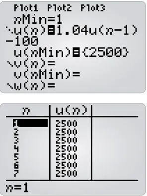
4.11

How to work with composite

functions

If fand gare functions, the related functions with rules f(g(x)) and g(f(x)) are called composite functions. It follows that the maximal domain for a composite function is at most the domain of the inner function. However, as the inner function is evaluated first, its value is substituted into the outer function, and this can only work if this value is an element of the domain of the outer function. So the range of the inner function must be a subset of the domain of the outer function for the composition to be defined. Hence the implied domain of a composite function is the domain of the inner function or a subset of this domain.

E

E x a m p l e

For the functions fand gwith rules below, state their implied domains. Also give the maximal implied domains of the composition functions with rules

f(g(x)) and g(f(x)), state their rules in simplified form, and plot the graphs of

y= f(g(x)) and y= g(f(x)).

a f(x) = x3, g(x) = cos(x)

b f(x) = x2, g(x) =

x

Solution

a The implied domain of each function is R, so each composition is also defined over domain R.

Press

o

Type Y1=X^3

¸

Type Y2=

™

(X)

¸

The first composition rule is f(g(x)) = (cos(x))3= cos3(x).

Type Y3=Y1(Y2)

¸

Press

q

, select 7:ZoomTrigand press

¸

The graph intersects the x-axis at the same places as the graph of

y= cos(x), as expected. Maximum and minimum points are also at the expected places.

The second composition rule is g(f(x)) = cos(x3).

Press

o

Alter the rule to Y3=Y2(Y1)and press

¸

Press

s

This looks weird! The difficulty is due to the fact that intercepts become more and more frequent (when x3= π/2, 3π/2, 5π/2 etc.) than for cos(x), and the limited number of pixels on the calculator screen makes it difficult to get a good plot.

Calculator software makes it easy to plot the graph of the ruleof a composite function directly, but care must be taken with domain restrictions. Your calculator can perform substitution and

simplification of rules but it cannot handle domain restrictions. You must determine the necessary restrictions yourself.

J

(32)

Press

p

and enter the following values:

Xmin = –3

Xmax = 3

Xscl = 1

Ymin = –1.5

Ymax = 1.5

Xres = 1

Press

s

We get a better view, showing how the effect of the inner function is to compress the graph of y= cos(x).

b For (ii), the implied domain of fis Rand the implied domain of gis [0, ∞).

The range of fand gare both [0, ∞) (check their graphs). Then ran

gdom f, so the composition f(g(x)) is defined on domain [0, ∞) =

domg. Similarly, ran fdom g, so the composition g(f(x)) is defined on

R= dom f.

Press

o

Type Y1=X^2

¸

Type Y2=

y

[

√

](X)

¸

The first composition rule is f(g(x)) = x.

Press

o

Type Y3=Y1(Y2)

¸

Turn off the plot of Y1 and Y2 (by pressing

¸

over the ‘=’ on these lines).

Press

q

¸

Note that the composite function is only plotted for [0, ∞).

The second composition rule is g(f(x)) = |x|.

Press

o

Type Y3=Y2(Y1)

¸

Press

s

Since the domain here is R, no restriction is necessary.

4.12

How to work with functional

equations

Functional equations are equations involving unknown functions that have to be found. Two examples are f(kx) = kf(x), where kis a constant, and f(x+ y) =

(33)

E

E x a m p l e 1

Consider the functional equation f(2x) = 2f(x).

a Show graphically that the circular function sinedoes not satisfy this functional equation.

b Check graphically which, if any, of the following function types satisfy this functional equation:

(i) a linear function whose graph passes through the origin (ii) a quadratic function whose graph has its vertex at the origin (iii) the exponential function with rule f(x) = ex_.

Solution

a Press

o

Type Y1=

˜

(X)

¸

Type Y2=Y1(2X)

¸

Type Y3=2

Y1(X)

¸

over the ‘=’ on the Y1 line)

Press

q

, select 7:ZoomTrigand press

¸

It is now clear that the two expressions are not identical, so sinedoes not satisfy the equation f(2x) = 2f(x).

b (i) To define a linear function with a graph through (0, 0), using y= xas an example:

Press

o

Type Y1= X

¸

Type Y2=Y1(2X)

¸

Type Y3=2

Y1(X)

¸

The two expressions are identical for all values in the viewing window, and it can be shown algebraically that linear functions of this type satisfy the equation f(2x) = 2f(x).

(ii) To define a quadratic whose graph has vertex (0, 0), using y= x2as an example:

Press

o

Type Y1= X^2

¸

Type Y2=Y1(2X)

¸

Type Y3=2

Y1(X)

¸

(34)

We can easily see that the two expressions are not identical, and it can be shown algebraically that quadratics of this type do not satisfy the equation f(2x) = 2f(x).

(iii) To define the exponential:

Type

Y1=e^(X)

¸

Type Y2=Y1(2X)

¸

Type Y3=2

Y1(X)

¸

(35)

5.1

How to calculate average and

instantaneous rates of change

The average rate of change for a function on [a, b] is .

Alternatively, it can be calculated using where his an

increment added to a given x value. The easiest way to do this with your TI-83/84 is to define your function, and then use this notation in subsequent calculations.

E

E x a m p l e

a Find the average rate of change for the function between the following values:

(i) x = 2 and x = 2.1 (ii) x = 2 and x = 2.05

(iii) x = 2 and x = 2.001

b Use the above results to find the instantaneous rate of change at x= 2.

Solution

a Press

o

Type Y1=X^2

You can now just use function notation to derive each average rate of change, as they all involve the same function.

Now determine the rate of change for each case individually.

(i) In this case, x = 2 and h = 0.1.

Type (Y1(2.1)–Y1(2))÷0.1

¸

The answer is 4.1.

f x

( )

= x2 f x h f x

h

+

(

)

−

( )

f b f a b a

( )− ( ) −

f x

( )

(36)

(ii) In this case, x = 2 and h = 0.05.

Type

(Y1(2.05)–Y1(2))÷0.05

¸

The result is 4.05.

Note: It may be quicker to edit the previous expression than to retype it.

(iii) In this case, x = 2 and h = 0.001.

Type (Y1(2.001)–Y1(2))÷0.001

¸

The result is 4.001.

As the increment, h,gets smaller, the average rate of change approaches 4. As happroaches zero, the average rate of change approaches 4.

b To find the value of the instantaneous rate of change at x = 2, find the limit of the average rate of change as happroaches zero. From a, it seems that this limit is 4.

So the instantaneous rate of change at x= 2 is 4.

(Note: this is what is referred to as the derivativeat x= 2.)

5.2

How to calculate the numeric

derivative

The numerical derivative gives you an approximation for the gradient of a tangent to a curve at a given x-value. This value is given by determining the average rate of change for a very small value of h. You can find the numerical derivative of a function using the graphing menu of your TI-83/84.

E

E x a m p l e

Find the value of the numerical derivative of at .

Solution

First produce a graph of the function .

Press

o

Type Y1=X^2

¸

Press

q

This plots the graph in a [−10, 10] by [−10, 10] window.

The standard viewing window is appropriate in this case.

y = x2

x = 3

5

(37)

To find the value of the numerical derivative:

Press

y

[CALC], select 6:dy/dx

and press

¸

When returned to the

s

screen, type 3÷5

¸

The cursor is now positioned on the curve at x 3

5. The value for the numerical derivative is 1.2.

Note: The nDeriv command can be used to calculate the numeric derivative

from the home screen. For example nDeriv (Y1, X, 3/5) could be used here.

5.3 How to calculate and plot

derivative functions

Using the numerical derivative feature, the TI-83/84 is able to plot gradient (or derivative) functions for a defined function rule. The command

nDeriv(Y1,X,2)

calculates the derivative of the function Y1 at x= 2. Entering

Y1=nDeriv(Y1,X,X)

gives a ‘plottable’ derivative function rule with respect to the variable x, for all values of x in the current viewing window.

In the example below, the ‘original’ function will be defined by the rule

Y1 = 0.1X(X – 6)(X+6)

.

E

E x a m p l e

If f(x) = 0.1x(x+ 6)(x– 6),

a Plot f(x) in the viewing window [–10,10] by [–10,10].

b Plot derivative function f '(x).

c Use the graphs to find the slope of f(x) at x= 2.1.

d Calculate the derivative of f(x) at x= 3.7 (from the HOME screen).

Solution

a Press

o

Type Y1=0.1X(X+6)(X–6)and press

Í

.

Press

q

, select 6:ZStandard.

This plots the graph in the window [–10,10] by [–10,10].

(38)

b Press

o

and type the function rule.

Press

m

, select

8:nDeriv to access the numerical derivative

function.

Type Y2=nDeriv(Y1,X,X)

Press

s

.

c Press

r

and

D

to select the derivative function in Y2.

Type 2.1and press

Í

.

This shows that that the gradient of f(x) at x= 2.1 is approximately –2.28. This can be verified by calculating the value of dy/dxon the original function in Y1 (as follows).

Press

r

and

D

to select the derivative curve.

Press

y

[CALC], select 6:dy/dx.

In the

s

screen, type 2.1and press

Í

.

So the gradient of the curve at x= 2.1 is approximately –2.28.

d Press

y

[QUIT]

to display the HOME screen.

Press

m

, select 8:nDerivto access the numerical derivative function.

Type nDeriv(Y1,X,3.5) and press

Í

.

5.4 How to draw tangent lines

The tangent line to a curve at a given x value can be calculated, and the equation of this tangent shown.

E

E x a m p l e

If f(x) = 0.1x(x+ 6)(x– 6),

a plot f(x) in the viewing window [–10,10] by [–10,10]

(39)

Solution

a Press

o

Type Y1=0.1X(X+6)(X–6)and press

Í

.

Press

q

This plots the graph in the window [-10,10] by [-10,10].

b Press

r

to select the curve.

Press

y

[DRAW], select 5:Tangent(

When prompted for the x value, type 5and press

Í

The curve is then drawn, and the equation is y= 3.9x– 25.

5.5 How to calculate the definite

integral

For a function, f(x) the definite integral is

b

a

f(x)dxF(b)F(a) where

F(x)

f(x)dx. On the TI-83/84, the function ‘fnInt’ with syntax [fnInt

(Y1,X, lower bound, upper bound)]

is used to calculate the value of

the definite integral.

E

E x a m p l e

Find the values of the following definite integrals:

a

4 1

dx

b Represent this integral graphically

Solution

a Press

y

QUIT to display the HOME screen.

Press

m

, select

9:fnInt( to access the numerical integral function.

Type fnInt(X2

÷5,X,1,4) and press

Í

.

x2

(40)

b Press

o

Type

Y1=X

2

÷5

and press

Í

.

Press

q

This plots the graph in the window [–10,10] by [–10,10].

Press

r

to select the curve.

Press

y

[CALC]

and select 7:

f(x)dx

When prompted for the lower limit value, type 1.

When prompted for the upper limit value, type 4.

The region representing the integral will then be shaded and the value of the integral calculated and displayed at the bottom of the screen.

5.6

How to find the area between

two curves

If f(x)g(x) in a given restricted domain[a,b], then the area between the two curves is found by calculating

b

a(f(x)g(x))dx. The area between a curve and the x-axis can be found numerically on the graph screen, or exactly on the home screen using the definite integral discussed in the previous section.

E

E x a m p l e 1

Find the area between the curve yx2and the x-axis for 0x3.

Solution

Press

o

Type Y1=X^2

¸

Press

q

¸

To find the area:

Press

y

(CALC), select 7:

∫

f(x)dx

and press

¸

When prompted for ‘Lower Limit’, type 0

¸

When prompted for ‘Upper Limit, type 3

¸

(41)

For the functions with rules f(x)8x2and g(x)x22: a graph fand gin a suitable window

b find the points of intersection between the graphs

c find the area between the curves.

Solution

a Plot the graphs to check which curve lies above which.

Press

o

Type Y1=8-X^2

¸

Type Y2=X^2+2

¸

Press

q

¸

The plot shows that f(x)g(x) between the points of intersection.

b To find where the two graphs intersect, you could use the graphical “intersect” command, or find the roots (zeros) of the function with rule

f(x)g(x) Press

o

Type Y3=Y1-Y2

¸

Using a variety of methods, it can be shown that the roots of this function are at x

3

orx

3

.

c Since f(x)g(x), the enclosed area is given by

3

((8x2)(x22))dx

Press

s

Press

y

(CALC), select 7:

∫

f(x)dx

and press

¸

When prompted for ‘Lower Limit’, type

3

¸

When prompted for ‘Upper Limit, type

3

¸

The area is approximately 13.85 (or 8

3

)

This value can be calculated at the home screen as well using the fnInt function (see right)

5.7

How to calculate the average

value of a function

The average value of a function over the domain [a,b] is given by

b a

f(x)dx. You can calculate this in one line using your

calculator.

E

E x a m p l e

1

ba

(42)

Press

y

QUIT

Press MATH and select 9:fnInt(

First enter , which is , and then the integral:

Type 1/5*fnInt(3X^2,X,0,5)

¸

The average value of this function is 25.

5.8

How to calculate and use the

second derivative

The second derivative, f(x) , is a useful tool for analysing the nature of a function’s stationary points. It is calculated using a similar syntax to that used in calculating the first derivative (nDeriv function from the MATH menu), using the nested syntax nDeriv(nDeriv(function rule, variable,

value, variable, value).

E

E x a m p l e

For the polynomial function with rule p(x)0.05(x1)3(x2)(x3)2: a Find the coordinates of all the stationary points.

b Calculate the value of the second derivative for each of these points.

c Use the value of the second derivative to determine the nature of each of the stationary points, and check your answer by plotting the graph in a suitable window.

d Find the coordinates of any non-horizontal points of inflexion.

e Find the coordinates of the point where p(x) in the domain x[1,3] is increasing most rapidly, and find the angle the graph makes with the positive x-axis at this point.

Solution

a First define the function as p(x):

Press

o

Type Y1=0.05

(X+1)^3

(X–2)

(X–3)^2

¸

To find the stationary points, use the methods outlined in Section 2.3 of this Toolkit. Using these or other methods, it can be found that the stationary points occur at (–1, 0), (0.76, –1.7), (2.40, 0.28), (3, 0)

1

₅

1

(43)

Type

y

QUIT

Type

Y3({-1,0.76,2.40,3})

¸

This yields the results:

f(1)0, f(0.76)3.42, f(2.40) 3.41, andf(3)6.4

c In summary,

At x 1, f (x)0 andf(x)0, ∴more information is needed (for example, plot the graph near x= -1)

x0.76, f (x)0 andf(x)0,∴local minimum

x2.40, f (x)0 andf(x)0,∴local maximum

x3, f (x)0 andf(x)0,∴local minimum.

d Non-horizontal points of inflexion require that f(x)0 andf 0. First solve f(x)0 for x:

Press

o

Turn off the plot of Y1 and Y2 (by pressing

¸

over the ‘=’ on these lines)

Press

s

to view the graph of f(x).

Press

y /

and select 2:zeroto find where f(x)0 The results are f(x)0 if x 1,0.02,1.60, and 2.75.

We can discount x 1since this is a stationary point of inflexion.

To find the y-coordinates for the others:

Type Y1({-0.02,1.60,2.75})

¸

This yieldsy{0.87,0.69,0.12}, so the coordinates of the non-horizontal points of inflection are

(0.02,0.87),(1.60,0.69), and (2.75,0.12).

e From the previous part, you will notice that the inflexion point at

x1.6 marks the steepest part of the curve in the domain x[1,3].

To find its gradient at this point:

Press

y

QUIT

Type Y2 (1.6)

¸

The result is f (1.6)1.91.

To convert this to an angle in radians:

Type

y

[TAN

–1

] 1.91

¸

This can be converted to degrees as shown.

(44)

This chapter covers the analysis tools on the TI-83/84 for representing and interpreting univariate statistical data.

6.1

How to store and summarise

ungrouped univariate data

In this section, we look at the entry of univariate data into lists, and the calculation of summary statistics for each list variable. The data is ungrouped in the following example.

E

E x a m p l e 1

The annual rainfall in a particular country town has been recorded over the last 20 years. The results, in millimetres, are:

146.8, 383.0, 90.9, 178.1, 267.5, 95.5, 156.5, 180.0, 90.9, 139.7, 200.2, 171.7, 187.2, 184.9, 70.1, 58.0, 84.1, 55.6, 133.1 and 271.8

a Go to the Stats/List Editor and clear any previously entered data, then enter the new data into List1.

b Calculate the five-figure summary (minimum, Q1, median, Q3 and maximum) for the sample.

c Ninety-five per cent of annual rainfall figures are expected to lie within two standard deviations of the mean rainfall. Use this sample data to calculate the upper and lower limits within which we can expect the annual rainfall figures to lie.

Solution

a Press

…

(EDIT), select 1:Edit

The Stats/List Editor screen displays list values in a column format (labelled L1, L2etc).

(Note: to clear a list, select the column heading and press

M

¸

.)

Enter the 20 values for the rainfall in the L1 column.

(45)

Press

…

(CALC)

and select 1:1-Var Stats Type 1-VarStats L1

The summary statistics for the data in L1 are displayed.

b The five-figure summary values are al