A space-time process model for the evolution of DNA sequences.

(1)

A Space-Time Process Model

for

the Evolution

of

DNA Sequences

Ziheng Yang

Department of Zoology, The Natural History Museum, London SW7 5BD, United Kingdom and College of Animal Science and Technology, Beijing Ap‘cultural University, Beijing 100094, China

Manuscript received April 29, 1994 Accepted for publication October 8, 1994

ABSTRACT

We describe a model for the evolution of DNA sequences by nucleotide substitution, whereby nucleotide sites in the sequence evolve over time, whereas the rates of substitution are variable and correlated over sites. The temporal process used to describe substitutions between nucleotides is a continuous-time Markov process, with the four nucleotides as the states. The spatial process used to describe variation and dependence of substitution rates over sites is based on a serially correlated gamma distribution, i.e., an autegamma model assuming Markov-dependence of rates at adjacent sites. To achieve computational efficiency, we use several equal-probability categories to approximate the gamma distribution, and the result is an autcdiscrete-gamma model for rates over sites. Correlation of rates at sites then is modeled by the Markov chain transition of rates at adjacent sites from one rate category to another, the states of the chain being the rate categories. Two versions of nonparametric models, which place no restrictions on the distributional forms of rates for sites, also are considered, assuming either independence or Markov dependence. The models are applied to data of a segment of mitochondrial genome from nine primate species. Model parameters are estimated by the maximum likelihood method, and models are compared by the likelihood ratio test. Tremendous variation of rates among sites in the sequence is revealed by the analyses, and when rate differences for different codon positions are appropriately accounted for in the models, substitution rates at adjacent sites are found to be strongly (positively) correlated. Robustness of the results to uncertainty of the phylogenetic tree linking the species is examined.

C

OMPARISON of homologous DNA sequences from

living species has provided an important tool for studying molecular sequence evolution. FELSENSTEIN

( 1981 ) described a maximum likelihood framework for modeling the process of nucleotide substitution combined with phylogenetic tree estimation. The model suggested by FELSENSTEIN assumes constant rate of substitution among nucleotide sites. This assumption has long been recognized as unrealistic, especially for genes that code for proteins or sequences that are otherwise functional (see WAKELEY 1993 and references therein )

.

The most important reason appears to be that different sites perform different structural and functional roles in the gene and are therefore under different selective constraints; this leads to variable rates of substitution at sites. Mutation rates may also be variable in different regions of the genome ( WOLFE et al. 1989).

There have been many attempts to account for rate variation among sites in nucleotide-substitution models. For example, JIN and NEI ( 1990) and TAMURA and NEI

( 1993) used the gamma distribution with given parameters to describe variable rates at sites when they constructed formulae for estimating the distance between two homologous DNA sequences. The gamma-distribu-

Address fw correspondence: Institute of Molecular Evolutionary Genet- ics, 328 Mueller Lab, University Park, PA 16802.

Genetics 139 993-1005 (Februaly, 1995)

tion model has also been extended to a joint likelihood analysis of all sequences by YANC (1993), which is a direct extension of FELSENSTEIN’S ( 1981 ) model of a single rate for all sites. Unfortunately the computation required by this method is very intensive, and YANC

(1994) suggested the use of a discrete distribution as an approximation to the (continuous) gamma. Use of the gamma distribution to describe rate variation among sites has been found to produce quite good fit to various data sets (see, e.g., WAKELEY 1993; YANC 1994; YANC et al. 1994)

.

The existence of “conservative” and “variable” regions in a gene suggests that rates of substitution may be not only variable, but also correlated, as sites within the same region may have similar rates characterized by the structural and functional importance of the whole region. In this paper, we will develop models that allow for such correlation by assuming Markov dependence of rates at adjacent sites. Such models will provide an alternative hypothesis for testing rate constancy and independence over sites, will produce more accurate prediction of rates at sites and will be useful for studying the effects of rate variation and correlation on various aspects of phylogenetic analysis.

(2)

994 Z. Yang

pendent over sites and are characterized by a spatial process. Our emphasis is on the spatial process used to model variation and dependence of rates over sites, but the temporal process of nucleotide substitution will first be described to introduce the necessary notation. The models will be applied to data of a segment of the mitochondrial genome from several primate species. We emphasize comparison of models, estimation of parameters and prediction of rates for sites as means for understanding the mechanisms of molecular sequence evolution.

THEORY

We consider substitutions only and ignore insertions and deletions. The data consist of S homologous DNA sequences from living species, each of N nucleotides long, and can be represented by an S X N matrix, X

= { xSn], where

x,,

means the nth nucleotide in the sth sequence; x,, takes a value from 1, 2, 3 or 4, represent- ing the four nucleotides, T, C, A or G, respectively. We use x, to denote one column in X , which is the nucleotide composition in different species at the nth site. It is apparent that x, is one of 4 X 4 X * * * X 4 = 4“ possible “site patterns” (see, e.g., GOLDMAN 1993). The species (and their representative sequences) are related according to an evolutionary tree; an “unrooted” tree topology for four species (

S

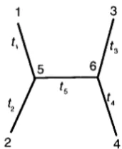
= 4 ) is shown in Figure

1, which will be used as an example to develop the theory. The sequences for extinct common ancestors, e.g., those at nodes 5 and 6 in the tree of Figure 1,

existed in the past and are now unknown. The sequences are assumed to evolve independently of each other after the separation of the species.

1 3

2 4

FIGURE 1.-An unrooted tree topology with four species used to develop the theory. The branch length is measured by the average number of nucleotide substitutions per site that have accumulated along the branch.

We assume that, for each site in the sequence, there is an overall rate of substitution that is determined by the structural and functional role of the site in the gene. This assumption appears legitimate when the sequences are not very different and homologous sites in different sequences perform more or less the same roles. YANG

(1993, 1994) considered the case where rates for sites are variable but independent; in this paper, we extend the theory to allow for correlation of rates at adjacent sites. We assume that conditional on the rates, substitutions occur independently at different sites. This is referred to as the conditional independence.

The temporal process: the Markov process model of nucleotide substitution: Nucleotide substitution is assumed to follow a (stationary) homogeneous Markov process, the four nucleotides being the states of the process. Let Q = {

a,,)

be the rate matrix of the process for a site with an average overall rate. We use the substitution model proposed by HASEGAWA et al. ( 1985), by which

1

7r 7‘ 7r c

where (&,,At ( y f u ) is the probability that nucleotide p changes into u in a small time interval

At.

Parame- ters nu’s give the equilibrium distribution of the process, with

X

T,, = 1, and we assume that the process is in equilibrium. Parameter K (usually

>

1 ) allows transi- tional substitutions ( T ++ C, A tf G) to occur with higher rates than transversional substitutions ( T, C ++ A, G)

.

The model will be designated “HKY.” The row sums of Q are 0; this allows the matrix of transition probabilities in time t to be calculated as P ( t ) = {Pfiu( t ) ] = exp( tQ) (see, e.g., GRIMMETT and STIR- ZAKER 1992, pp. 239-246). As t and Q occur in the form tQ only (in the likelihood function) , we choose the scale factor f = 1

/

[ 4 ~ ( nT7rC;

+

T ~ ? T ~ ; )

+

4 ( 7 r T

+

7 r c ) ( r A

+

T ~ ; ) ] , so that the average rate of substitution is 1 when the process is in equilibrium, i.e.,

-E

7r,Q,

K T A - ( KTA

+

n-,-

+

T C )

= 1. Q thus represents the pattern of nucleotide substitution whereas the overall amount of evolution is reflected in t. Time t, or the branch length in a tree, is then measured by the expected number of nucleotide substitutions per site that have occurred during the time interval or along the branch. We do not assume the constancy of substitution rates among lineages, an assumption known as the molecular clock; as a result, the placement of the root in a tree will not affect the likelihood; that is, only unrooted tree topologies can be identified ( FELSENSTEIN 1981 )

.

To calculate P ( t ) = exp( tQ) ,we perform the spec- tral decomposition (diagonalization) of Q ; if Q =

U

-

diag{ A I ,

Az, AJ,

A4) U ” , then P ( t ) = U *

(3)

DNA

U “

,

where the As are the eigenvalues of Q and col- umns of

U

are the corresponding (right) eigenvectors; those for the HKY model are given by HASEGAWA et al.

(1985).

The overall rates for sites are assumed to be random variables, either independent or Markov dependent, as will be described later. If the rate for site n is r, ( n =

1, 2,

. . .

, N) , the rate matrix for the site will be r,Q, and the matrix of transition probabilities for the site will be P (r,t) = exp( r,tQ)

. Suppose that the nucleotide

composition for this site is x, = (XI, Q,

x$,

xq]’ (we

have written xln, Q,, * * * as xl, Q , *

- -

for conciseness)

.

The conditional probability of observing x,, given the rate for the site r,, is (YANG 1993)

4 4

f(xnlm) =

c c

7 r ~ p ~ x , ( r , t l ) p x . ~ ~ ( r , ~ )

x5=l q = l

x

~ x 5 q ( r , t 5 ) p ~ X ~ ( r , ~ ) p ~ x / , ~ r , t 4 ) . (2)

The “root” of the tree, i.e., the starting point for calculation, is (arbitrarily) fixed at node 5 in the tree of Figure 1, and 7 r x 5 is the probability of observing nucleo-

tide

x5

at node 5, given by the equilibrium distribution of the process. The summations are taken over the unknown nucleotide states (

x5

and %) in the extinct ancestors at nodes 5 and 6. For an arbitrary tree topology of many species, this conditional probability can be effi- ciently calculated using the postorder tree-traversal algorithm of FELSENSTEIN ( 1981 )

.

The spatial process: Markov chain transition in the auto-discrete-gamma model of rates over sites: The gamma distribution with parameters a and

p

has mean

a

/

and variance a

/ p 2 .

Since the rate for site ( r ) is seen to be a scale factor, we set

p

= a so that K ( r ) = 1 (with variance 1

/

(Y )

.

The density function of ris then

g ( r ; a ) = a a r ( a ) ” e - a r r a ” , r > 0, a

>

0. ( 3 )

The single parameter a is reversely related to the extent of rate variation among sites. When a 2 1, the

distribution is fl-shaped; a + 00 reduces to the model of a single rate for all sites. When a

<

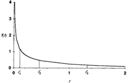
1, the distribution is highly skewed and has a L-shape, which suggests that most sites have very low rates of substitution or are nearly “invariable”, and yet there are a few mutational “hot spots”; the case of a = 0.5 is shown in Figure 2.

Maximum likelihood estimates of a from real data have been in the range 0.1 -1.0 ( YANG 1993; YANG et al. 1994)

.

Assuming independence of rates among sites, YANG

(1993) presented an approach to calculating f ( x,) = r ) ’ [ f ( x,I r,) ] and hence the likelihood function. Be- cause the computation required by this model is very intensive, YANG (1994) suggested a “discretegamma model” ( d G ) , whereby a discrete distribution is used to approximate the (continuous) gamma. The range of r (0, ”) is separated into K categories by K

+

1

4

3

(6 2

1

0

r

FIGURE 2.-Discretization of the (marginal) gamma distribution of rates for sites using four equal-probability categories [adapted from Figure 1 of YANG (1994)

1.

The distribution shown in the graph has parameter a = and is the

x’

distribution with one degree of frezdom. T$e boundar- ie2 for categories are calculated as r o = 0, r l = 0.1015,

r 2 = 0.4549, r : = 1.3233 and r,* = m , which are the per-

centage points corresponding to

p

= 0,

’//,,

‘//,, ‘//, and 1. The means of the four categories are

6

= 0.0334, 5 = 0.2519,

r3 = 0.8203 and 6 = 2.8944, respectively; these are used to represent all rates in each category.

-

threshold points, r o = 0, r l , r 2 ,

. . .

, rlfi =

03,

such that each category has probability 1

/

K of occurrence (Fig- ure

2)

.

The mean of a category is used to represent all rates in the category. We denote using the mean for the ith category, which covers the interval ( r i P l , r i )

.

For given value of parameter a , the threshold points r r s and the mean rates cs can be easily calculated

In this paper, we posit Markov dependence of rates over sites. Our implementation is through this discretized gamma distribution, resulting in an auto-discrete- gamma model of rates for sites. We start from consider- ing the auto-gamma model with rates taken as continuous random variables and then construct the discrete version as its approximation. For simplicity, we use a Markov chain to model the correlation of rates at neighboring sites; given the rate rmPl for site n - 1,

the distribution of rate r, at site n is specified fully. It appears more realistic and natural to have r, depend on rates at both its two neighboring sites, that is, on both r,_l and r , , ] , which means using a Markov random field to model rate variation along the sequence. How- ever, this is noted to add tremendous complexity to calculation of the likelihood function ( CRESSIE 1991, pp. 383-573) and is not attempted in this study. Need- less to say, we also ignore possible correlation of rates at sites separated by more than one nucleotide. We also consider an alternative model that assumes that r, depends on only instead of r,-l; this turns out to give identical results for the auto-discrete-gamma model of this paper.

Consider the rates R, and h$ for any two neighboring sites in the sequence, which are two (continuous) ran-

*

* *

*

(4)

996 Z. Yang

dom variables. As the marginal distributions of Rl and

&

are both gamma, Rl and R2 are known to follow a

bivariate gamma distribution (JOHNSON and KOTZ 1972,

p. 216). Many such distributions have been constructed (see e.g., JOHNSON and KOTZ 1972, pp. 216-230). For

mathematical tractability, we have chosen to use the one due to MORAN (1969). Let 2, and Z, be two random variables with a standard bivariate normal distribution whose density is

(27r) - 1 ( 1 - p 2 ) -1’2

Define random variables Ul and U2 by the equations

u,

= (27r)

1:

exp( -t‘/2) dt = (a(.&) ( 5 )

and Uz = (a(&). The marginal distributions of Ul and

U2 are both uniform (rectangle) in the interval (0, 1 )

.

Now define random variables Rl and R2 by the equations

U, = g( 7 ; a ) d 7 =

loR’

aar(

a ) - 1 e - a 7 7 a - 1 d r

= G ( & ; a ) ( 6 )

and U, = G ( & ; a ) .

The joint probability density of Rl and

&

are given by MORAN ( 1969 ) for the more general case that R1 and

&

have marginal gamma distributions with different

parameters. In our model, the spatial Markov process is assumed to be stationary, and Rl and

&

are assumed to have identical marginal distributions.

When we use K categories to approximate the marginal distributions of Rl and

&,

the correlation between R1 and

&

will be modeled by the conditional probability that site n is from category j (with rate

5 )

,

given that site n - 1 is from category i (with rate T ; )

.

Let Y, be the rate category that site n is from. This probability will be Mtj = prob (Y, = j l YnP1 = i ) =

prob ( r , =

51

rnPl = E )

.

M = { Mtl] then constitutes the matrix of transition probabilities for a Markov chain, the states of which are the Krate categories. We calculate M g as following:

Mv = prob (Y, = j l Y,-] = i )

*

2 prob(r,-]

<

&

<

r i

* *

I

r i - ]

<

Rl

<

r ? )

Using ( 5 ) a n d ( 6 ) , these probabilities (integrals) can be easily mapped onto the Z, -

&

plane. The problem turns out to be the calculation of the cumu- lative distribution function of a standard bivariate normal distribution, that is, Q 2 ( z l , G , p ) = prob (2,

<

zl, Z,

< +)

.

There appears to have been much

repetition and confusion in the statistics literature concerning approximate methods for calculating Q 2 . We have employed the method of OWEN (1956), based on the FORTRAN implementations of it by DONNELLY ( 1973) and YOUNG and MINDER (1974)

(see HILL 1978; THOMAS 1979; CHOU 1985; BOYS 1989 for remarks on YOUNG and MINDER’S program). The results are checked against appropriate tables published in Biometrika around 1930. The matrix M calculated in this way is symmetrical; this may be a short- coming of the model rather than an advantage with respect to its fit to data. However, this property, together with the stationarity assumption of the Markov chain, assures that the same likelihood function is obtained no matter whether we let r, depend on r,-l only or on T , , ~ only. The equilibrium distribution of

the Markov chain specified by M has equal probability

( 1

/

K) for each rate category, in congruence with the (discretized) marginal distribution of Rl and R2. The model is referred to as an auto-discrete-gamma model of rates for sites (“Ad,”).

The correlation, pc = corr ( Rl , &) , between the two (continuous) gamma-distributed variables, is positively related to parameter p, which is p = corr ( Zl , $) , although an algebraic relationship between the two seems difficult to obtain. The correlation ( p d G ) between the rates at two neighboring sites in the autodiscrete- gamma model can be calculated as following for given values of parameters a and p.

prob ( YnPl = i ) M - F F ‘I ‘ I - 1

P d G =

Cf=l prob(Y,-l = i) * y: - 1

1

Cf=]

Zfll

* M $ q - 1

-

1

’=’

K E

( 8 )

CK

“ . f - 1

where prob ( Y,-l = i) = 1

/

Kaccording to the marginal distribution of rates for sites; the mean of the distribution is 1:

EE1

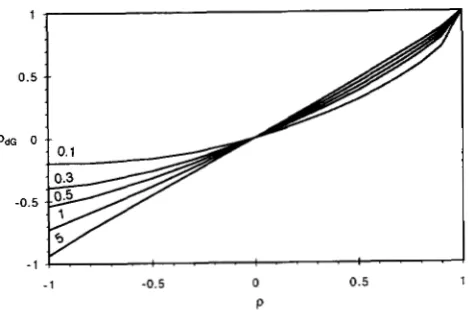
prob(Y,-l = i ) - E = Ccfil 1/K. 5;. = 1.

The relationship between parameter p ( 4 ) and pdG ( 8 ) is depicted in Figure 3. When p = 0, we have pc = P d G = 0, Mq = prob (Y, = j ) = 1

/

K, and the model reduces to the discrete-gamma model with independent rates for sites.

The likelihood function: Parameters in the autodis- Crete-gamma model include 8 = { 7 r T , 7rc, 7 r A , K , a, p } , which are common to different tree topologies, and t

= ( tl ,

t

,

t3, t 4 , t 5 ] , which are branch lengths in a specific tree topology (Figure 1 ) . Note that the joint distribution of Yl

,

Y 2 ,

. . .

,

YN is

prob(Y1 =

3 ,

Y2 =

B,

. . .

,

YN = YN)

(5)

DNA 997

- 1 -0.5 0 0.5 1

P

FIGURE 3.-The relationship between pdG ( 8 ) and parameter p (4) . The curves are for different values of the a parameter: 0.1, 0.3, 0.5, 1 and 5.

where we set prob ( Yl = yl ) = 1

/

K , due to the stationarity of the chain. With the assumption of conditional independence of data over sites given the rates, the likelihood function is

w ,t;

x )

= prob ( X ; 8, t )

-

*

i

(prob(Yl = y l , Y2 = 8 , .

. .

,

YN = y N ) K

Y l = l Y N ‘ 1

N

X

II

f(

XnI rn =

7”)

n=l

where f( x,] r, =

qe)

is given in

( 2 ) .

As the summa- tion signs in (10) can be moved rightward, a simple algorithm is possible for calculating the likelihood function. Let b, ( n ) = prob ( x n , x,+1,

. . .

, xNI Y, = i) be the probability of observing data x,, x,+],

. .

.

, xN, given that site n is from rate category i. Then

K

bi(?L) =f(xnIrn =

E )

Mq.bj(n

+

1 ) (11)

,= 1

with b, ( N ) = f( xNI rN = E ) . The likelihood is simply

L = prob(Yl = i ) - b i ( l ) . (12)

The computation required by this model is then only slightly more than that for the discrete-gamma model assuming independent rates for sites, which is roughly K times that required by a model assuming constant rate for all sites. As a common practice, we

K

i = l

estimate the parameters r T , rc and T A in the HKY

model ( 1 ) by using the averages of the observed nucleotide frequencies in the sequences. Other parameters are estimated by maximizing the likelihood function. In theory, any numerical optimization algo- rithms can be used for this purpose, and an EM algorithm for this type of model was described by LEROUX and PUTERMAN (1992). In this paper, a quasi-Newton algorithm is used to obtain estimates of parameters by iteration, with the gradients calculated using the difference method.

Accounting for rate differences at different codon positions: Sometimes sites in the sequence can be naturally grouped into different classes, which are known to change at different rates. This is the case for protein-coding DNA sequences, where the three codon positions are known to change at quite different rates due to the different selective constraints exerted on them; mutations at the third position may not cause changes of the amino acids whereas those at the second position always do. Another possibility is when several genes (of the same species) are combined into one data set, and different genes can be assumed to evolve with different rates determined by their relative conservativity. It seems reasonable to assign different rate parameters for sites from such different classes. If there are g site classes, we can assume that sites from class j ( j = 1,

2,

. . .

, g) have rate ci, with c1 = 1; the cs are rate ratios. We will very loosely refer to such site classes as “codon positions” and designate models that use different rates for different classes of sites as “C”.

The rate matrix for a site which is from the j t h site class and which has a gamma-distributed rate r

is then r c j Q , with transition probability matrix P ( t )

= exp ( r c , t Q )

.

The likelihood function can be calculated as before, although the treatment of the cs is different from that of the rs. Simply, rates for codon positions are parameters and rates from the gamma distribution are random variables. Given any site, we know which codon position it is from and hence its rate parameter c,. However, we do not know what value of r corresponds to the site. The likelihood function is obtained by summing over all possibili- ties for the random variables rs but not over the parameters c s .

Prediction of substitution rates at sites: We study the conditional distribution of rates for sites (the T S ) given

the data ( X )

.

With the assumption of independent rates over sites, YANC and WANC (1994) have noted that use of the conditional mean, 9 = E ( rl x ) , as the predictor of the true rate ( r ) for a site with data x

maximizes the correlation between the predictor and the true rate. Specifically, for any other predictor P =

(6)

998 2. Yang

the auto-discrete-gamma model, this can similarly be defined as

f, = E(r,IX) = E(rnlxn, x,+1,

. . .

,

XN)

X;=,

T*prob(Y, = 2)-

N

- prob(x,, x,+,,

. . .

,

xNI Y, = i)

prob(x,, x,+,,

. . .

, XNI Y, = 2)

prob (Y, = i)

-

- E-prob(Y, = i). b j ( n )

(13) prob(Y, = i). b i ( n )

where prob (Y, = i) = 1

/

K , and 6, ( n ) is defined in

(11) and calculated at the maximum likelihood estimates of parameters. Alternatively, the mode of the conditional distribution may be used, which will result in the maximum

a

posterior predictor. This means using E

as the predicted rate for site n, by which i maximizes

f(

x,

I

r, =

E )

or bi ( n ) for the discretegamma model or auto-discrete-gamma model, respectively. However, this is found to be less, and sometimes much less, effi- cient than use of the conditional mean for the discrete- gamma model assuming independence of rates over sites (results not shown) , presumably because the conditional distribution ( r,

I

x,) is most often highly skewed and the mode of the discrete distribution is not very representative of the whole distribution. The mode of the a f m o r (continuous) distribution ( 3 ) does not exist

for a

<

1. We expect this to be true also for Markov-

dependent rates over sites, and use (13) to predict rates. Rates calculated according to ( 13) are normally not equal to any of the cs ( i = 1,2,

.

,

K ) ; we suggest that this is justifiable as we consider the discrete gamma model as an approximation to the continuous gamma.

Nonparametric models of rates over sites: We have also considered models for variable rates over sites, either independent or Markovdependent, without assuming a specific distributional form for the rates. Sim- ply, the discretegamma model’s Es and J;s, which used to be functions of parameter a , and the auto-discrete- gamma model’s Es and Mqs, which used to be functions of parameters a and p , are now taken as free parameters. Let K be the number of categories of rates. Such a model includes 2 ( K - 1 ) free parameters when rates over sites are assumed to be independent; these are the frequencies for the rate categories:

fi

,

k,

. . .

,

f , - , (f,

is not a free parameter as Z J; = 1 ) and the rates for the categories

c , q ,

F ~ - ~ (-,is given by the requirement C J E = 1 ) . The nonparametric model assuming Mar- kov dependence will involve ( K

+ l

) ( K - l ) parameters. These are the rates for the categories

5 ,

Q ,

. . .

,

T ~ - ~ , and the K X K elements of the matrix M with the restriction that the K row sums of M are all one; the frequencies for categories (the J s ) are given by the equilibrium distribution of the Markov chain specified by M .

Clearly the nonparametric models formulated above involve many parameters, especially when more than two rate categories are considered. We therefore consider another version of these models, with the restriction that each rate category has equal probability of occurrence. With independent rates for sites, this means ( K - 1 ) free parameters (the 7 s ) ; with Markov dependence, this restriction means that both the row sums and the column sums of M are one and M is known as a double stochastic matrix; the model then in- volves K ( K

-

1 ) parameters.

Maximum likelihood estimation of parameters in these models and prediction of rates by (13) can pro- ceed in a way similar to the auto-discrete-gamma model described before.

ANALYSIS OF PRIMATE MITOCHONDRLAL DNA (mtDNA) SEQUENCES

Data: BROWN et al. ( 1982) determined the sequences of a segment of the mitochondrial genome from human, chimpanzee, gorilla, orangutan and gibbon. There are 896 nucleotide sites in the sequences except that orangutan has a nucleotide missing at position 560. The beginning part of this segment (nucleotides 1-

458) codes for part of protein ND4 (NADH-dehydroge- nase subunit 4 ) and the ending part (nucleotides 658-

896) codes for part of protein ND5 (NADHdehydroge- nase subunit 5 ) . The middle of the segment (nucleotides 459-657) codes for three tRNAs, i.e., histidine, serine and leucine tRNAs (BROWN et al. 1982) . Se- quences of this region are now also available for several other primates, and we have added those for crabeating macaque, squirrel monkey, tarsier and lemur ( HAYA- SAKA et al. 1988) , so that the expanded data set contains nine species. The sequences were aligned by A. FRIDAY. Several sites in the tRNA-coding region involve gaps (insertions or deletions) , and these are excluded, with 888 nucleotides left in each sequence. We note that possible errors in the alignment or the removal of sites involving gaps may bias the analysis, because consecu- tive sites in the resulting data may not in fact be direct neighbors, as is assumed in the models of Markov-dependent rates for sites. However, we expect such bias to be small for the current data set, as the sequences are very similar so that the alignment appears quite reliable and only a few sites in the tRNA-coding region are removed.

(7)

squirrel monkey

gibbon

human \ o m 4 r ' l w v

orangutan

tarsier

/

0.278 gibbon

0.175

orangutan 0.230

crab-eating macaque

\

lemur

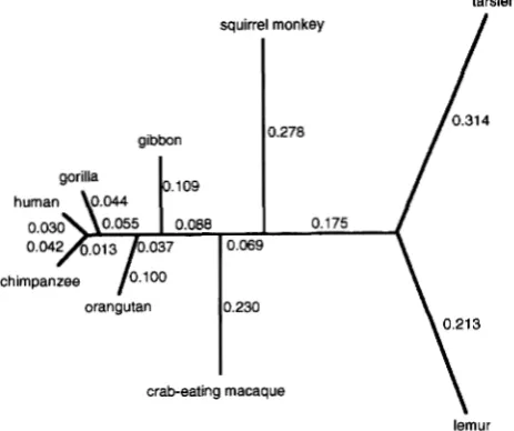
FIGURE 4.-The phylogenetic tree for nine primates whose mtDNA sequences (888 bp) are analyzed in this paper. Branch lengths shown in the tree are calculated under the HKY+C+AdG model, measured as the average numbers of substitutions per site at the first codon position. This tree topology ( b u t not the branch lengths) is assumed to compare models and predict rates for sites in the paper.

frequencies in the whole sequences are ;irT = 0.266, 7ic = 0.304, 7 i A = 0.322 and ;irG = 0.108, and these are taken as estimates of the frequency parameters in the HKY substitution model ( 1 )

.

Nucleotide frequencies in different species, either for the whole sequence or at different codon positions, are similar, which suggests that the temporal processes of nucleotide substitution are more or less homogeneous and stationary. However, nucleotide frequencies at different codon positions are quite different; for example, the frequencies are 0.209

( T ) , 0 2 7 3 ( C) ,0.385 ( A ) , 0.133 ( G) at the first codon position whereas they are 0.179 ( T ) , 0.413 ( C )

,

0.365 ( A ) , 0.042 ( G) at the third position. Our models assume one common

Q

(and thus one set of frequency parameters) for all the codon positions and are not adequate in this respect. It is possible to modify the models to allow for this feature by using different frequency parameters in the HKY model for sites from different codon positions; this is not pursued here, and we suggest that our analyses of rate variation along the sequence will not be influenced much by this inaccu- racy of the models.

The phylogenetic relationship among the species may be represented as the tree shown in Figure 4. There exists controversy about the positions of tarsier and lemur (A. FRIDAY, personal communication) , but this is concerned with only the placement of the root in the tree. The humanchimpanzee-gorilla separation does not seem to be very controversial anymore, and general opinion appears to support the ( (human, chimpanzee), gorilla) relationship. We will use the tree topol-

ogy shown in Figure 4 to estimate parameters, compare models and predict rates. The effects on these analyses due to the uncertainty of the phylogenetic relationship will be discussed later, together with the problem of estimating the phylogeny using different models.

Estimation of parameters from the parametric mod- els: The auto-discrete-gamma model reduces to the model of a single rate for all sites when there is only one rate category ( K = 1 )

.

When K -+ a, the model

will approach the (continuous) auto-gamma model. We expect that the likelihood values and parameter estimates will change dramatically for small values of K, but when Kis sufficiently large, the results will stabi- lize. YANG ( 1994) analyzed several quite different data sets using the discrete-gamma model assuming independent rates over sites; different values of Kwere used, including the (continuous) gamma model of YANG

( 1993) which corresponds to K =

00.

Such comparisons suggest that four rate categories can provide optimum or near-optimum fit by the model to data and also quite good approximation to the (continuous) gamma distribution as reflected by the estimated a parameter. In this paper, we have introduced Markov dependence of rates into the models, but have not implemented the (continuous) auto-gamma model ( K = a). Instead we perform all analyses using two values of K ( 4 a n d 8 ) to get some feel about the effect of K. The results, i.e., likelihood values, parameter estimates and predicted rates obtained from using these two values of K turn out to be quite similar, which suggests that four categories may be sufficient for the auto-discrete-gamma model for analyzing real data, just as in the case of the discretegamma model ( YANC 1994)

.

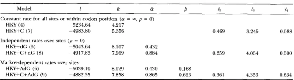
In the following, we present results obtained by using K = 8, with com- ments given on those obtained from using K = 4.

Log-likelihood values and parameter estimates obtained under different models are shown in Table 1.

The simplest model (HKY) assumes a single rate for all sites, which gives log-likelihood 1 = -5234.64 with

k = 4.217 ? 0.292 (standard errors are obtained by inverting the matrix of second-order derivatives of the log-likelihood with respect to parameters, calculated by the difference method). Either assuming discrete- gamma rates for sites (HKY+dG) or using different rate parameters for codon positions (HKY+C) leads to tremendous improvement in likelihood, suggesting the existence of severe rate variation among sites in the sequence. In fact, neither the discretegamma model nor the rates for codon positions alone can account for the rate variation observed in these data, since HKY+C+dG is significantly better than either HKY+dG (comparison of 2 4 1 = 251.62 with

x:,

P

<

0.01) or HKY+C (comparison of 2Al = 131.94 with

x:,

P

<

(8)

1000 Z. Yang

TABLE 1

Log-likelihood values and parameter estimates under different parametric models

Constant rate for all sites or within codon position ( a = a, p = 0)

HKY (4) -5234.64 4.217

HKY+C (7) -4983.80 5.356

Independent rates over sites ( p = 0) HKY+dG (5) -5043.64 8.107 0.432 HKY+C+dG (8) -4917.83 7.969 0.884

0.469 3.245 0.588

0.359 4.054 0.500

Markov-dependent rates over sites

HKY+AdG (6) -5039.10 8.029 0.430 0.168

HKY+C+AdG (9) -4882.35 7.858 0.865 0.623 0.361 4.353 0.634

Values in parentheses are the numbers of free parameters in the models, not including branch lengths. Parameters are

estimated assuming the tree topology of Figure 4, and estimates of branch lengths are not shown. The frequency parameters in the HKY model (nl, 7 r c ; and xA) are estimated by using the averages of observed frequencies in the sequences. Models with dG assume (independent) discretegamma rates over sites, whereas those with AdG assume the autodiscrete-gamma rates; K = 8 rate categories are used in both cases. Models with C assume different rate parameters for codon positions: c, = 1, G ~ , c3 and c4 for sites at the first, second and third codon positions in the protein-coding regions and for those in the tRNA-coding region, respectively.

coding region are quite different. They are in the proportion q :

6:

4.:

t4 = 1:0.359:4.054:0.500 by the HKY+C+dG model, ie., the third codon position changes >10 times faster than the second, and also sites in the tRNA-coding region change more slowly than the first codon position in the protein-coding regions. Furthermore, different sites at the same codon position also have quite different rates of substitution. The estimate of a under the HKY+C+dG model ( & =

0.884 t 0.124) is larger than that under HKY+dG ( &

= 0.432 2 0.043) ; this is obviously because the rate parameters for codon positions (the c s ) in the HKY+C+dG model have explained substantial part of the rate variation. However, estimates of rate parameters for codon positions (the c s ) remain more or less the same whether or not the (discrete) gamma model is assumed to account for the remaining rate variation. Parameter K and branch lengths (not shown) are se-

verely underestimated when rate variation among sites exists but is ignored in the models, as observed by Y ~ G

et al. (1994) ; also WAKELEY 1994).

Use of the HKY+AdG model assuming Markov dependence leads to & = 0.430

+-

0.044 and ,5 = 0.168 -C

0.056. These values of a and p give pd(; = 0.121 by ( 8 ) . Although ,5 is significantly greater than 0 , the serial correlation is not very strong. (The likelihood ratio test for the null hypothesis of rate independence over sites, i.e., p = 0 , means comparison of 2A3 = 9.08 with X : ,

P

<

0.01). Nevertheless, when rate differences at the

codon positions are accounted for in the model (HKY+C+AdG) , the estimate of p is much higher, i.e., ,5 = 0.623 2 0.060; this value of p , together with & =

0.865

-+

0.124, gives pdC; = 0.544 by ( 8 ) . The increase in log-likelihood by introducing auto-correlation is also

much greater; i.e.,

2AZ

= 70.96 ( P

<

0.01). These results suggest very strong correlation of rates at adjacent sites. The reason for the difference between the two estimates of p is that before accounting for rate differences at codon positions (HKY+AdG) , rates at sites three nucleotides apart are highly correlated, so that the correlation between rates for two adjacent sites is weakened (see results concerning predicted rates for sites below).

Using four rate categories ( K = 4 ) rather than eight in the above comparisons would give essentially identical results. The estimates of parameters are also very similar. For example, those obtained from the HKY+C+AdG model ( K = 4 ) are ri = 7.843, & = 0.866,

,5 = 0.665,

&

= 0.361, Z3 = 4.361, Z, = 0.639, with 1 =

-4883.67 ( cJ: Table 1 ) . When K = 1, 2, 3, 4, 8 and

20,

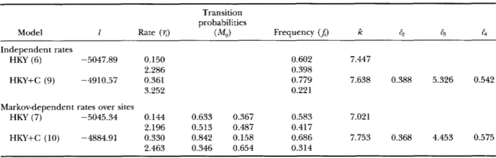
the log-likelihood for the HKY+C+AdG model is

(9)

TABLE 2

Log-likelihood values and parameter estimates under the nonparametric models with two rate categories

Transition probabilities

Model 1 Rate ( T ) ( M y ) Frequency

(A)

ri 62 63 4

Independent rates

HKY (6) -5047.89 0.150 0.602 7.447

HKY+C (9) -4910.57 0.361 0.779 7.638 0.388 5.326 0.542

2.286 0.398

3.252 0.221

Markovdependent rates over sites

HKY (7) -5045.34 0.144 0.633 0.367 0.583 7.021

2.196 0.513 0.487 0.417

2.463 0.346 0.654 0.314

HKY+C (10) -4884.91 0.330 0.842 0.158 0.686 7.753 0.368 4.453 0.575

See note to Table 1.

gamma models assuming independence (results not shown). This seems to be due to two reasons. First, adding parameters ( p in this case) to a model will normally “decrease” the accuracy of estimates of other parameters. Second, the positive correlation of rates at sites implies positive correlation of data at sites, which will cause the data to contain less information than if they are independent. In sum, ignoring correlation of rates over sites when it exists does not seem to bias estimates of other parameters too much, but the calculated standard errors in the estimates will give a wrong impression of high accuracy.

The nonparametric models: We have fitted the nonparametric models to the mtDNA data, assuming either independence or Markov dependence of rates over sites. The parameter-richness of the models has led to many problems when more than three rate categories are used; these will be discussed later. The results shown in Table

2

are obtained using two rate categories ( K =

2 )

.

Overall the same conclusions can be drawn from these results as from those in Table 1. For example, Table 2 clearly suggests that rates of substitution are different for sites at different codon positions and for different sites from the same codon position (results for models assuming a single rate for sites are listed in Table 1 ) . The most complex model, which assumes different rate parameters for codon positions and Mar- kov-dependent random rates over sites, is significantly better than all the simpler models. The likelihood Val- ues are so different that we do not need to consult statistical tables to perform the tests. According to this model, rates for the first, second, third codon positions in the proteincoding regions and for sites in the tFWA-coding region are in the proportion 1:0.368: 4.453:0.575. Furthermore, the remaining rate variation can be best explained by two rates 0.330, 2.463,

with

stationary probabilities 0.686 and 0.314, respectively.

Estimates in the M matrix suggest that if a site is in rate category one, the next site will have probability 0.842

of being in category one too and probability 0.158 of switching into category two, whereas if a site is in category two, the next site will remain in category two with probability 0.654 and switch to category one with probability 0.346; thus rates at neighboring sites are positively correlated. Using parameters (the c s ) to account for rate differences at codon positions is seen to reduce the remaining rate variation (as indicated by the smaller differences between and 6 ) , and to considerably increase the correlation of rates at neighboring sites (as reflected by larger M I , and M Z 2 ) . These results are con- gruent with those obtained from the auto-discrete- gamma models (Table 1 ) . Estimates of the rates (the

c s ) and frequencies (the J s ) are more or less stable whether independence or Markov dependence is assumed for rates over sites. Estimates of parameters K

and the cs are also very similar to those obtained from the corresponding discrete-gamma models (Table 1 )

.

Results obtained from the nonparametric models under the restriction that each rate category has equal probability of occurrence are presented in Table 3. Be- cause of this restriction, we have been able to obtain results with either 2 or 3 rate categories. The frequency for each category is J =

‘ / n

or ‘ / s for K = 2 or 3, respectively. Note that models with two rate categories

( K = 2 in Table 3 ) are equivalent to the corresponding (auto-) discrete-gamma models with two rate categories;

5

and M1, in the current models correspond to a

and p in the auto-discrete-gamma models through a reparameterization. Again, the most complex model is

(10)

1002 Z. Yang

TABLE 3

Log-liielihood values and parameter estimates for the nonparametric models

~

Model 1 Rate (5;) Transition probabilities (m,J R

r,

q l:d

Independent rates

HKY (5) -5052.21

HKY+C (8) -4924.87

Markovdependent rates

HKY (6) -5047.60

HKY+C (9) -4890.47

Independent rates

HKY (6) -5044.01

HKY+C (9) -4914.54

Markov-dependent rates HKY (10) -5024.08

HKY+C (13) -4879.31

Two equal-probability categories of rates

0.110 1.890 0.254 1.746

0.109 0.576 0.424

1.891 0.424 0.576

0.253 0.791 0.209

Three equal-probability categories of rates

0.031 0.408 2.561 0.314 0.314 2.372

0.164 0.972 0.000 0.028

0.191 0.000 0.484 0.516

2.645 0.028 0.516 0.456

0.217 0.869 0.087 0.044

0.424 0.022 0.644 0.334

2.359 0.109 0.269 0.622

6.394

7.664

6.284

7.712

8.176

7.763

7.262

7.915

0.370

0.373

0.364

3.804

4.150

4.709

4.683

0.518

0.644

0.530

0.666

Values and estimates given for models under the restriction of equal probability in each rate category using two or three rate categories.

Tables 1 or

2

are also apparent in Table 3. Estimates of K and the cs are quite similar to those in Tables 1

and 2. The models with two or three rate categories (Table 3 ) are not nested so that a likelihood ratio test cannot be applied to compare them, but it seems that three rate categories are worthwhile.

The problem of phylogenetic trees: FEISENSTEIN (1981; see also FELSENSTEIN 1973; THOMPSON 1975)

suggests that the likelihood values calculated for different tree topologies can be compared to estimate the phylogenetic relationship among the species. The method is known as maximum likelihood estimation of the phylogenetic tree. Estimation of phylogeny from DNA sequences has been of great interest to evolutionary biologists, and one may (rightly) require that an adequate model be used in such an adventure. This paper focuses on construction and comparison of models as means for understanding the processes of DNA

sequence evolution. Strictly speaking, comparison of models, especially by using the chi-square approximation to the likelihood ratio test, requires the likelihood values to be calculated (and parameters to be estimated) using the true phylogenetic relationship ( Z .

YANG, N. GOLDMAN and A. FRIDAY, unpublished data). In practice, the difficulties involved in these two interre- lated problems are quite different. In the following, we give a short discussion on the implications of results of this study to the two problems.

First, our ignorance or uncertainty concerning the phylogenetic relationship does not seem to introduce much error in the estimation of parameters in the evolutionary models or in the comparison of such models. There are 1 X 3 X

- -

-

X ( 2 X 9 - 5 ) = 135,135 possible bifurcating tree topologies for nine species. To see the effects of changes to tree topologies, we have performed all analyses described above using several other tree topologies although results obtained from the tree of Figure 4 only are presented (Tables 1 - 3 ) .

As an example, we list in Table 4 the likelihood values and parameter estimates obtained under the HKY+C+AdG model for these tree topologies. The nine-species star tree has only nine branches. Other tree topologies used differ from the tree of Figure 4 only concerning the human-chimpanzee-gorilla separation. Let T , = ( ( H C ) G ) represent the tree of Figure

(11)

Space-Time Model for DNA Evolution

TABLE 4

Log-likelihood values and parameter estimates under the HKY+C+AdG model for several different tree topologies

Tree 1 R & ij

4 Q

4

Star tree -5016.46 15.358 0.346 0.455 0.214 5.466 0.527

TI = ((HC)G) -4882.35 7.858 0.865 0.623 0.361 4.353 0.634

Tz = ((HG)C) -4888.44 7.827 0.861 0.621 0.366 4.426 0.654

Tq 1 ((CG)H) -4885.96 7.660 0.893 0.628 0.372 4.456 0.648

To = (HCG) -4888.45 7.825 0.861 0.621 0.366 4.428 0.654

((HG)C),T3=((CG)H)andTo=(HCG),Tohav-

ing a trifurcation. The star tree is quite different from

To,

T I , T2 or

T3,

and estimates of parameters obtained for this tree are admittedly quite different from those for other trees. However, parameter estimates obtained for To,

T,

,

T2 or

T3,

which are not too wrong and may all be called “reasonable” trees, are very similar. Likelihood values for different trees are not very different, especially in comparison to the dramatic changes in likelihood due to changes in the assumed models (see Tables 1, 2 and 3 ) . The same pattern is observed for other models considered in this paper (see YANG et

al. 1994 for more examples). This means that we will obtain essentially the same results concerning parameter estimation and model selection, no matter which of the reasonable trees is used.

In contrast, the small differences in likelihood among tree topologies suggest the difficulty of phylogenetic tree estimation; some of the theoretical difficulties are discussed by Z. YANG, N. GOLDMAN and A. FRIDAY (unpublished data). It has been observed that ignoring rate variation over sites can substantially influence phylogenetic tree reconstruction, especially the estimation of branch lengths (YANG et aZ. 1994; also WAKELEY 1994). Nevertheless, this study tends to suggest that ignoring the correlation of rates over sites will not influence phylogenetic tree reconstruction greatly, at least if the point estimation only is concerned. For all models considered in this paper, the order of the likelihood values for the examined trees has been IT,

>

lTS

>

lT2

>

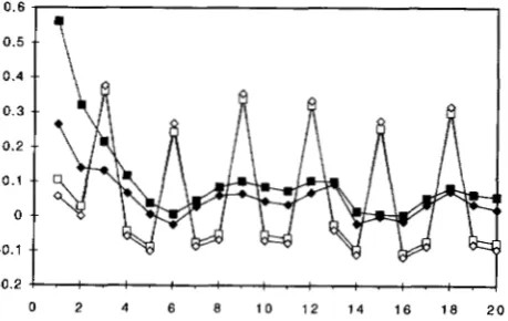
lTo; it seems very likely that T I (Figure 4 ) is the maximum likelihood tree by these models if all tree topologies could be evaluated. We suggest that for the estimation of tree topology, the discrete-gamma model is elaborate enough, and the auto-discrete-gamma model may not be worthwhile.

Prediction of rates at sites: We calculated the rates for the 888 sites in the mtDNA sequence using (13) based on maximum likelihood estimates of parameters in the models. As another way to look at rate dependence over sites, we calculated the serial correlations using the predicted rates and the results are shown in Figure 5. The correlation (0.562) of predicted rates at two adjacent sites calculated from the HKY+C+AdG

model ( K = 8 ) agrees well with P& = 0.544 calculated from ( 8 ) using the maximum likelihood estimates of the parameters, Li = 0.865 and j3 = 0.623 (Table 1 ) .

The decrease of the serial correlation with the number of nucleotides that separate the sites also agrees nicely with the model’s expectation. The predicted rates can be plotted along the sequence after some smoothing and appear very useful for identifylng conservative and variable regions in the sequence (results not shown). The period of three in the curves for the HKY+dG and HKY+AdG models is clearly due to these models’ failure to account for rate differences at the codon positions. In this regard, the “detrending” or removal of the large scale variation by using rate parameters for codon positions in the HKY+C+dG and HKY+C+AdG models is seen to be quite successful. We also note that the serial correlations, especially those for sites that are separated by one or two nucleotides, calculated from the HKY+C+dG model, which assumes independent rates over sites, are smaller than those obtained from

0.6

0.5

/

1

0 2 4 6 8 1 0 1 2 1 6 1 4 1 8 20

FIGURE 5.”Serial correlation of substitution rates along the mtDNA sequence, which are predicted by assuming the HKY+C+AdG (M) , HKY+C+dG ( ) , HKY+AdG ( 0 ) and HKY+dG ( 0 ) models; K = 8 categories are used in these discrete-gamma models. The tree topology of Figure 4 is as-

(12)

1004 2. Yang

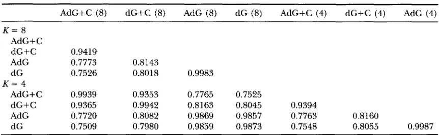
TABLE 5

Correlations between rates predicted from different (auto-)discrete-gamma models

using eight or four categories

AdG+C (8) dG+C (8) AdG (8) dC (8) AdG+C (4) dG+C (4) AdC (4)

K = 8 AdG+C

dG+C 0.9419

AdC 0.7773 0.8143

dG 0.7526 0.8018 0.9983

AdG+C 0.9939 0.9353 0.7765 0.7525

dG+C 0.9365 0.9942 0.8163 0.8045 0.9394

AdG 0.7720 0.8082 0.9869 0.9857 0.7763 0.8160

dG 0.7509 0.7980 0.9859 0.9873 0.7548 0.8055 0.9987

K = 4

the HKY+C+AdG model, which assumes Markov dependence. The results from the HKY+C+AdG model are clearly more reliable, and suggest that if one (wrongly) assumes rate independence over sites in the model, one will underestimate the extent of dependence, which is not very surprising.

Table 5 lists the correlations between rates predicted using different methods. If we consider the HKY+C+AdG model as giving the best predicted rates for sites, these correlations will indicate the relative efficiency of rate prediction by other models. Rates predicted using four categories have correlations -0.99 with those using eight categories. Combined with the similarity of likelihood values and parameter estimates for these two values of K , we suggest that four categories are sufficient for analyzing real data. Rates predicted from models assuming independence (the dG models) are closely related to rates predicted from corresponding models assuming Markov-dependence (the AdG models)

.

We also note that using one of the tree topologies T 2 , T3 or To instead of T I produces very similar predicted rates (results not shown). Similar to the results of YANG and W m c ( 1994), possible errors in estimates of parameters or tree topologies normally do not affect the accuracy of rate prediction much.

DISCUSSION

The spatial-process models considered in this paper have many counterparts in various fields of applied statistics, especially in analyses of time series or spatial data. In time-series analysis, the counts of events that occur in fixed time intervals have a Poisson distribution (with the variance equal to the mean) when the process is generated by a constant homogeneous rate. When the underlying rate is variable, it is known as an over- dispersed process, since the variance of the counts is larger than the mean. When the rate is itself an independent gamma variable, the counts are known to follow a negative-binomial distribution. The nonparamet-

ric models considered in this paper are known as jinite- mixture models as the data are generated from a mixture of categories of rates with different probabilities. With Markov dependence, the models are also known as hid- den-Markov-chain models, as the states of the chain are random variables and are not observable. LEROUX and

PUTERMAN ( 1992) summarized recent developments of techniques concerned with the finite-mixture models. CHURCHILL ( 1989) employed a hidden-Markov-chain model to describe the occurrences of nucleotides in a single DNA sequence. The distinction made in this paper between the rate parameters for codon positions (the c s ) and the gamma-distributed random rates (the

r s ) is analogous to the linear-mixed-models theory, which is widely used in animal breeding (HENDERSON

1973), although the current models are highly nonlin- ear; rates for codon positions are fixed effects, for which we estimate their main effects (the c s )

,

whereas rates from the gamma distribution are random effects, for which we estimate their variance components (parameters

a and p ) and predict rates (the r s ) based on the observed data.

(13)

by LEROUX and PUTERMAN ( 1992) in their analysis of a sequence of counts of movements by a fetal lamb. For example, estimates obtained by those authors from a Markov-dependent mixture model with four rate categories suggest that there exists an absorbing state in the Markov chain with rate 0, which means that as soon as the fetus enters this rate category, it will never move again; because the chain is assumed to be stationary, this also means that the fetus has been and will remain motionless. We have been able to obtain equally absurd results using our nonparametric models with three or four rate categories.

The auto-discrete-gamma model (HKY+C+AdG in Table 1 ) and the two versions of nonparametric models assuming Markov dependence (Tables 2 and 3 ) are not nested, and so the likelihood ratio test is not directly applicable for comparing them. However, the likelihood values suggest that the auto-discretegamma

model provides a better fit to the data than the nonparametric models using two rate categories. When three categories are used, the nonparametric models (e.g.,

the last model listed in Table 3 ) can fit the data slightly better than the autodiscrete-gamma model, but at the cost of many more parameters. It is also noteworthy that results obtained using two or three categories in the nonparametric models are not easily comparable, but K is not an important factor in the auto-discrete- gamma model as long as a relatively large value (such as four) is used. We conclude that the auto-discrete- gamma model provides the most-parsimonious explana- tion of rate variation at sites in these mtDNA sequences.

C source codes are available from the author which implement models described in this paper.

I thank CLIVE MONCRIEFT for many useful discussions about the bivariate gamma distributions. This study was partially supported by a grant from the Natural Science Foundation of China.

LITERATURE CITED

BOB, R. J., 1989 Remark AS R76: a remark on algorithm AS 76: an

probabilities. Appl. Statist. 38: 580-582.

integral useful in calculating non-central t and bivariate normal

BROWN, W. M., E. M. PRAGER, A. WANG and A. C. WILSON, 1982 Mitochondrial DNA sequences of primates, tempo and mode of evolution. J. Mol. Evol. 18: 225-239.

CHOU, Y.-M., 1985 Remark AS R55: a remark on algorithm AS 76: an integral useful in calculating non-central t and bivariate normal probabilities. Appl. Statist. 34: 100-101.

CHURCHILI., G . A,, 1989 Stochastic models for heterogeneous DNA sequences. Bull. Math. Biol. 51: 79-94.

CRESSIE, N. A. C., 1991 Statistics for Spatial Data. John Wiley and Sons, New York.

DONNEI.LY, T. G., 1973 Algorithm 462: bivariate normal distributions. Comm. ACM 16: 638.

FEUENSTEIN, J., 1973 Maximum likelihood and minimum-steps methods for estimating evolutionary trees from data on discrete characters. Syst. 2001. 22: 240-249.

FELSENSTEIN, J., 1981 Evolutionary trees from DNA sequences: a maximum likelihood approach. J. Mol. Evol. 17: 368-376. GOLDMAN, N., 1993 Simple diagnostic statistical tests of models for

DNA substitution. J. Mol. Evol. 37: 650-661.

GRIMMETT, G. R., and D. R. STIRZAKER, 1992 Probability and Random Processes, Ed. 5, Clarendon Press, Oxford.

HAYASAKA, R, T. GOJOBORI, and S. HORAI, 1988 Molecular phylogeny and evolution of primate mitochondrial-DNA. Mol. Biol.

HASEGAWA, M., H. KISHINO and T. YANO, 1985 Dating the human- ape splitting by a molecular clock of mitochondrial DNA. J. Mol.

HENDERSON, R., 1973 Sire evaluation and genetic trends, pp. 10- 41 in Animal Breeding and Genetics Symposium in Honour of Dr. J. L. Lush. American Society of Animal Science and Animal Dairy Science Association, Champaign, IL.

HILL, I. D., 1978 Remark AS R26: a remark on algorithm AS 76: an integral useful in calculating non-central t and bivariate normal probabilities. Appl. Statist. 27: 379.

JIN, L., and M. NEI, 1990 Limitations of the evolutionary parsimony method of phylogeny analysis. Mol. Biol. Evol. 7: 82-102.

JOHNSON, N. L., and S. KOTZ, 1972 StatisticalDistributions: Multivari-

ate Continuous Distributions. John Wiley and Sons, New York. LEROUX, B. G., and M. L. PUTERMAN, 1992 Maximum-penalized-

likelihood estimation for independent and Markovdependent mixture models. Biometrics 48: 545-558.

MOW, P. A. P., 1969 Statistical inference with bivariate gamma distributions. Biometrika 56: 627-634.

OWEN, D. B., 1956 Tables for computing bivariate normal probabilities. Ann. Math. Statist. 27: 1075-1090.

TAMURA, I C , and M. NEI, 1993 Estimation of the number of nucleotide substitutions in the control region of mitochondrial DNA in humans and chimpanzees. Mol. Biol. Evol. 10: 512-526. THOMAS, G. E., 1979 Remark AS R30: a remark on algorithm AS

76: an integral useful in calculating non-central t and bivariate normal probabilities. Appl. Statist. 28: 113.

THOMPSON, E. A., 1975 Human Euolutionaly Trees. Cambridge Uni- versity Press, Cambridge.

WAKELEY, J., 1993 Substitution rate variation among sites in hyperva- riable region 1 of human mitochondrial DNA. J. Mol. Evol. 37:

WAKELEY, J., 1994 Rate variation among sites and substitutional bias among nucleotides are conflated in simple sequence comparisons. Mol. Biol. Evol. 11: 436-442.

WOLFE, K. H., P. M. SHARP and W.N. LI, 1989 Mutation rates differ among regions of the mammalian genome. Nature 337: 283- 285.

YANG, Z., 1993 Maximum likelihood estimation of phylogeny from DNA sequences when substitution rates differ over sites. Mol. Biol. Evol. 10: 1396-1401.

YmG, Z., 1994 Maximum likelihood phylogenetic estimation from DNA sequences with variable rates over sites: approximate meth-

ods. J. Mol. Evol. 3 9 306-314.

YANG, Z., and T. WANG, 1994 Mixed model analysis of DNA sequence evolution. Biometrics (in press).

YANG, Z., N. GOLDMAN and A. E. FRIDAY, 1994 Comparison of models for nucleotide substitution used in maximum likelihood phylogenetic estimation. Mol. Biol. Evol. 11: 316-324.

YOUNG, J. C., and Ch. E. MINDER, 1974 Algorithm AS 7 6 an integral useful in calculating non-central t and bivariate normal probabilities. Appl. Statist. 23: 455-457. [Correction: Appl. Statist. 28:

113 (1979)l EvoI. 5: 626-644.

E d . 22: 160-174.

613-623.