Copyright 0 1996 hy the Genetics Society of America
On the Consistency of a Physical Mapping Method to
Reconstruct
a
Chromosome
in
Vitro
Momaio
Xiong,* Hubert J. Chen? Rolf
A.Prade,: Yuhong Wan
James Griffith,II
William
E. Timberlaken and Jonathan Arnold
P
*Department of Mathematics and Molecular Biology, University of Southern California, Los Angeles, California 90089, tDepartment of
Statistics, University of Georgia, Athens, Georpa 30602, $Department of Microbiology and Molecular Genetics, Oklahoma State University, Stillwater, Oklahoma 74078, §Department of Molecular Biology, Jilin University, Chang Chun 130023,
People’s Republic of China, “Department of Genetics, University of Georgza, Athens, Georgia 30602, and qMyco Pharmaceuticals, Inc., Cambridge, Massachusetts 02139
Manuscript received February 6, 1995 Accepted for publication September 15, 1995
ABSTRACT
During recent years considerable effort has been invested in creating physical maps for a variety of organisms as part of the Human Genome Project and in creating various methods for physical mapping. The statistical consistency of a physical mapping method to reconstruct a chromosome, however, has not been investigated. In this paper, we first establish that a model of physical mapping by binary fingerprinting of DNA fragments is identifiable using the key assumption-for a large randomly gener- ated recombinant DNA library, there exists a staircase of DNA fragments across the chromosomal region of interest. Then we briefly introduce epi-convergence theory of variational analysis and transform the physical mapping problem into a constrained stochastic optimization problem. By doing so, we prove epiconvergence of the physical mapping model and epi-convergence of the physical mapping method. Combining the identifiability of our physical mapping model and the epi-convergence of a physical mapping method, finally we establish strong consistency of a physical mapping method.
0
NE goal of the Human Genome Project is to cre- ate detailed maps of the human genome and of several other model organisms (COLLINS and GALAS 1993) as a prelude to determining their entire DNA sequence. The size of these genomes vary from a few million base pairs of DNA in a bacterial genome to over 3 billion base pairs in a mammalian genome. I n the last several years considerable progress has been made in mapping a diverse array of organisms ranging from bacteria to humans (COULSON et al. 1986; OLSON et al.1986; KOHARA et al. 1987; AZEVEDO et al. 1993; COHEN
et al. 1993; EIGLMEIR et al. 1993; HOHEISEL et al. 1993; MIZUKAMI et al. 1993; CAI et al. 1994). This progress has been made possible by a variety of new recombinant DNA methodologies (DAVIES and TILGHMAN 1990; BILL
INGS et al. 1991), which include cloning and automated sequencing of DNA fragments. The power of this tech- nology for generating mapping and sequencing data has fundamentally shifted the problem from one of collecting the mapping data to the inference problem of assembling the maps. It is the latter problem, which is the focus of this article.
A central statistical challenge of the Human Genome Project is assembling a physical map of a whole chrome some from a large number of DNA markers along a chromosome. A physical map represents a partial order-
ing of distinguishable DNA fragments by their position along a chromosome. While recombinant DNA technol- ogy provides a wealth of markers to distinguish DNA fragments for mapping, physical maps have existed since nearly the beginning of genetics. One of the simplest and oldest examples is a cytological map in fruit flies.
There is a wide variety of physical maps including cytological maps, radiation hybrid maps, STS content maps, ordered clone collections (i.e., “contig maps”), restriction maps, and the DNA sequence of an entire chromosome, reflecting the diversity of experimental approaches used to generate them. The focus of this report is on assembling one particular kind of physical map, an ordered clone collection. Even within this nar- rower class of physical maps, a rich variety of finger- printing methodologies exist for distinguishing clones in a library for the purpose of ordering this library. Some of these fingerprinting methods include the use of (1) restriction enzymes (COULSON et al. 1986; OLSON et al. 1986);
(2)
restriction enzymes supplemented with Southern hybridization to synthetic L1 and Alu se- quences (STALLINGS et al. 1990; BELLANE-CHANETELOT et al. 1992); (3) sequence-tagged sites (STSs) (GREEN and OLSON 1990a,b; FOOTE et al. 1992); (4) synthetic oligonucleotides (CRAIG et al. 1990; HOHEISEL et al.1991, 1993); and ( 5 ) low copy number DNA probes
Curresponding authm: Jonathan Arnold, Genetics Department, Uni- (MIZUKAMI et al. 1993; WANG et al. 1994a). The focus of
versity of Georgia. Athens. ” GA 30602. this paper will be on creating an ordered clone collec-
E-mail: [email protected] tion with fingerprinting methods that utilize “low copy
number” DNA probes that occur once or a few times in a genome [ i.e., methods (3) and ( 5 ) ] because these two methods are being used to create a high resolution physical map of the human genome over the next 5 years. These methods are also being used to create phys- ical maps of a variety of other organisms including Ara- bidopsis thaliana, Aspergdlus fumigatus, Candida albicans, Cryptococcus neoformans, Neurospora crassa, Staphylococcus
aureus, and Enterococcus faecium.
Modeling physical mapping experiments statistically and estimating their parameters, including the original order of the clones in the library, are important for planning a physical mapping project, evaluating infer- ence tools for map assembly, and for understanding the data from mapping experiments. In physical mapping by fingerprinting methods (1)
-
( 5 ) there is a stochastic process by which clones in a library are sampled as well as a stochastic process by which the DNA within each clone is sampled in order to fingerprint that clone. No matter which method of fingerprinting is used, proce- dures for physical mapping consist mainly of ordering random clones by their fingerprints in much the sameway
that “call numbers” might be used to order books in a real library. A mathematical description and statistical analysis of these processes have been proposed and used for designing physical mapping experiments, for identi- fylng overlaps between clones, and for ordering clones(LANDER and WATERMAN 1988; GRICORJEV and MIRONOV
1990; ARRATIA et al. 1991; BALDING and TORNEY 1991; BAIULLOT et al. 1991; KARLIN and MACKEN 1991; PALAZ-
ZOLO et al. 1991; TORNEY 1991; CUTICCHIA et al. 1992a;
Fu et al. 1992; ZHANG and MARR 1993; WANG et al. 1994a). For any particular fingerprinting method, it is not an easy task to order clones in a library. For n clones, the total number of possible orders is n!. GOLDSTEIN and WATERMAN (1987) considered the efficacy of a simu- lated annealing algorithm in assembling a restriction map. Unfortunately, they demonstrate that under a cer- tain probability model there is an exponentially increas- ing number of solutions as a function of the length of chromosome segment being mapped with probability 1. CUTICCHIA et al. (1992a) examine another approach to ordering clones in a library. Each clone is scored for the presence or absence of target DNA sequences by hybridization to a panel of probes, thereby assigning a digital call number to each clone. The number of differences between a pair of call numbers establishes a distance between clones. They formulated the clonal- ordering problem in terms of minimizing the sum of linking distances between successive clones as a function of their order along a reconstructed chromosome, i.e.,
the traveling salesman problem (TSP) (GAREY and JOHN- SON 1979) and computed a solution to the minimization problem using simulated annealing. Whether or not this estimator of the original order of the clones based on the data from physical mapping experiments is consistent
remains an open question and may depend on the iden- tifiability of an underlying physical mapping model.
The objective of this paper is to prove the consistency of an ordering procedure based on a physical mapping criterion, such as total linking distance (CUTICCHIA et al. 1992a). First, a description of the physical mapping data generated by methods ( 3 ) and (5) and a real exam- ple of an inferred physical map of an entire chromo- some are given in the EXAMPLE section. Second, a statisti-
cal model for the physical mapping process and a statistical method for reconstructing the order of clones in a library is developed in the MODEL section. A princi-
pal ingredient in the proof of consistency is the “identi- fiability” of this model. The definition of identifiability of a model and its proof for the physical mapping model are also included in the MODEL section. A nontechnical
statement of a consistency result for a physical mapping method is given together with a sketch of its proof and a statement of its biological implications in the CONSIP
TENCY section. The problem of ordering clones is then
formulated as a stochastic optimization problem under
METHODS, and the problem of proving consistency of
clonal ordering methods is translated into showing con- vergence of an optimal solution of a stochastic optimiza- tion problem to its true solution. Under METHODS a basic concept and a theorem of stochastic optimization are also briefly introduced. This theorem is then used to prove the consistency of a particular estimator of a li- brary’s true clonal order under RESULTS. Finally, in the
DISCUSSION some comments are made, and some direc-
tions for future research, indicated.
EXAMPLE
Several steps are involved in generating a physical map of a whole chromosome by fingerprinting methods in- volving the use of low copy number probes [methods ( 3 )
and (5)] : (1) intact chromosomal DNA is isolated (BRODY
et al. 1991);
(2)
isolated chromosomal DNA is physicallysheered or cut by restriction fragments into smaller frag- ments; (3) these smaller fragments are size-selected by gel electrophoresis into 40 kilobase (kb) fragments (or larger, depending on the size of the target genome); (4) size-selected DNA fragments are inserted into a cloning vector (e.g., WAHL et al. 1987) (i.e., a plasmid, phage, cosmid, or artificial chromosome). The result is a c h r e mosome-specific library of DNA fragments. The number of clones n in a library is designed to be large enough so that with high probability each base pair of chromosomal DNA is represented at least once in the library (ie., the expected coverage probability is near 1) (FU et al. 1992). Choice of library size is related to the genome size (N),
the cloning vector’s insert size (M), and the expected coverage probability. The resulting library is a sample of size n from the chromosome.
Physical Mapping Consistently 269
Raw data
Probes
NDEKAJFMBGHILC
13
...
.1....
08
..
1...
1...
16
...
.1..19
...
1...
1.01
...
.1.....
25 1
...
1......
12
..
1...
1..1....20
...
1...1.... 1.11
..
1...1..1....07
.
.l.....
22 1...
1......
03
....
1...1....
117
....
.1....
.1..23 1
...
.1......
09
..
1...
l... 26 1...
1....
05 .1..
...
10..
1...
l... 02...
.1.. .l.....
15...
.1....
04 .1... 1
....
124 1
...
l......
14...
.1....
18
....
.1....
.l.. 06 .1.....
21 1..1...
l.... 1.27
...
.1...
" """"""" " """"""" " """"""" Redundant order of clones Robes NDEKAJFMBGHILC 01
...
.1.....
02
...
.l.. .l.....
03....
1...1.... 104 .1... 1
....
105 .1..
...
06 ,l.....
" """"""-- " """"""" 07.
.1.....
08..
1...
l... 09..
1...1.......
10
..
1...
l... 11..
1...1..1......
order 12 13 1...1..1.......
.1....
".) 14
...
.1....
15
...
.1....
16
...
.1..17
....
.l....
.1..18
....
.l....
.1..19
...
1...
1.20
...
1...1.... 1.21 1..1...1.
...
1.22 1
...
l... 23 1...
l... 24 1....
..1......
25 1
...
1...
26 1
...
1....
27
...
.1...
" """_""" " """"""" Minimal order of probes Robes ABCDlEFGlHlIJlKLMN " " "" " ~ = = = ~ = ~ = = ~ = z = = " 01 l...I...I.I..I
....
02 11..
I...I.I..l....
03 111.1...
I.I..I....
04 .1111...
I .I..
I....
05...
11...
I . I . . I....
06...
11...
1 . 1 . . I....
"""_~"_~_~"~"~_
07....
Il..I .I.. I....
08....
111.1 .I.. I....
09....
111. I .I.. I....
10....
111.1 .I..I....
11....
1111l.l.. I....
12....
I111 I.
I.. I....
-
13....
I..ll.I..I....
14....
I ..lI. I.. I....
15....
I ..lI. I.. I....
_ " " " ( " _ ~ _ ~ " ~ _ _ " 16....
I...
I
.[I. I....
17....
I...
I .I111....
18....
I...
I. 1111....
_~""_~"_~_~"~""
19....
I...
I .I.. 111..20
....
I...
I .I.. 1111.21
....
I...
I. I.. Ill11 22....
I...I.I.. 1..1123
....
I...I. I..I ..1124
....
I...
1.I..
1..1125
....
I... 1.1.. 1..1126
....
I...I.I.. 1..11" ""1"_1_1"1""
27
....
I...
111..I
....
" ""1"-1-1"1""
Transpose
Reorder
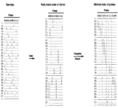
FIGURE 1.-Ordering clones and then probes converts the data marix into a physical map. The physical map is displayed as
a tweway layout with clones down the rows in their order along the chromosome and probes across the columns in their order along the chromosome. A 1 indicates clone/probe hybridization or equivalently, detectable overlap. A period indicates no clone/probe hybridization or equivalently, no detectable overlap.
MIZUKAMI et al. 1993; WANG et al. 1994a). The finger- printing process then involves taking a sample of m
probes and hybridizing them to n clones in a library. Selecting the number of probes m is discussed in FU et al. (1992). The result is a n X m binary data matrix (Figure l ) , in which 1 indicates hybridization and pe- riod, no hybridization. The probes can be randomly sampled from the primary library used for mapping
(HOHEISEL et al. 1993; MIZUKAMI et al. 1993; WANG et al.
1994a) or from a secondary library with smaller inserts (FOOTE et al. 1992). In the example of this section probes are sampled from the primary library (WANG et
al. 1994a). The resulting collection of m probes is a means to sample the DNA from each clone.
The resulting data are extremely simple, and the meth- ods above lend themselves to robotic data collection and to computer analysis. Each clone in the library corre- sponds to a row of the binary data matrix. Each probe sampled corresponds to a column of the data matrix. Contiguous blocks of clones or "contigs" are linked to- gether by their common hybridization pattern to a panel of probes. The physical mapping problem is then to uncover a permutation of the rows and columns that reveals the true ordering of clones and probes along the
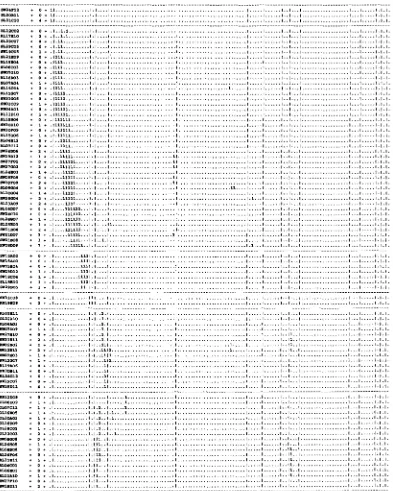
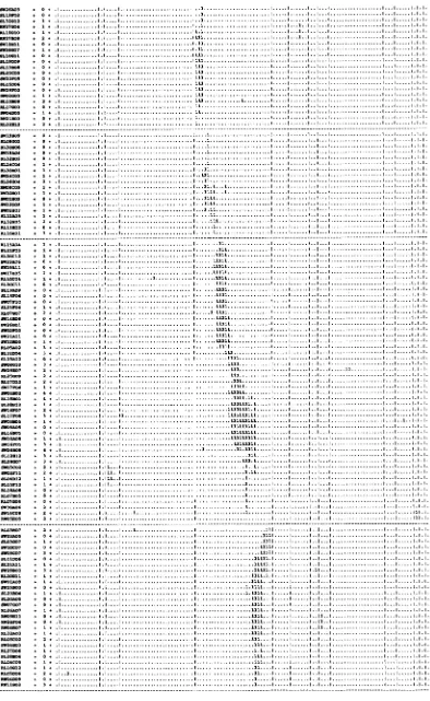
chromosome. This process is diagrammed in Figure 1. This process is analogous to the job of a librarian, namely examining a clone's binary call number (i.e., a row in Figure 1) and placing the clone next to other clones with similar call numbers. The distance between a pair of clones can be measured by the number of differences in their digital call numbers. One method of ordering the clones is simply to minimize the sum of the linking distances between adjacent clones in the data matrix by randomly permuting the rows (CUTICCHIA et al. 1992a). The same process can be applied to the transpose of the binary data matrix to order the columns. The end product of this process is a physical map of a whole chromosome (Figure 2, WANG et al. 1994a).
In this example a panel of 115 probes are hybridized to 593 clones from chromosome N o f a fungus, Asperg.ll-
lus nidulans. This ordered clone collection represents
an in vitro reconstruction of a 2.9 megabase (Mb) chro-
mosome. The horizontal lines demarcate 31 contigs, a sequence of 1 or more clones, each overlapping with its neighbor(s). The vertical lines demarcate 12 cells,
m r m + o + II.... ... I.I....I.. ... I...I...I...I..I...I...I...I...I.I.I. S W O B l 1 f 0 f 11 ... 1.1 .... I...I...,l...l...l..l...,...l...l...l.l.l.
S L 3 1C 10 I 4 f 11 ... 1 . 1 .... I... ... I... ... l...l...l..l...l...l...l...~.l~l.l.
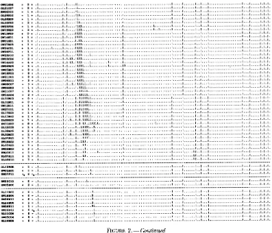
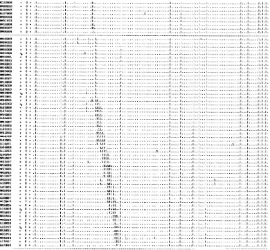
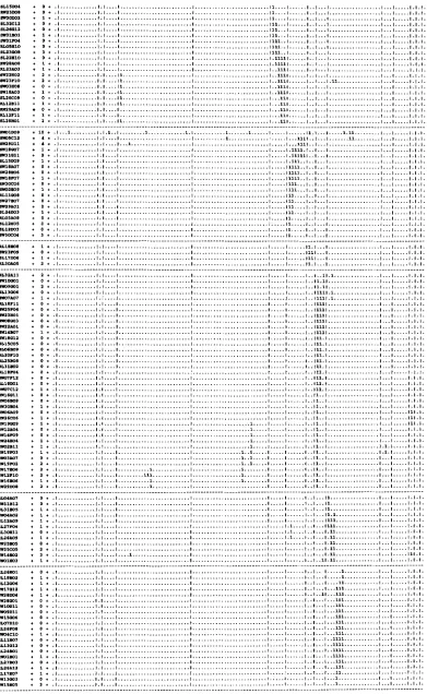
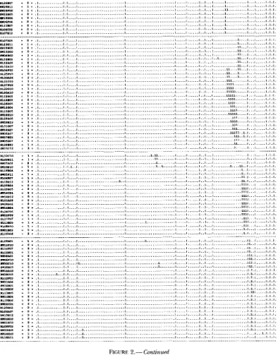
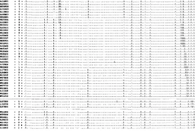
FIGURE 2.-Physical map of chromosome W i n A. nidulans. The chromosomal map was constructed by minimizing the total linking distance D with the random cost algorithm (WANG et al. 1994a). Clone names are given in the margin of the map in their inferred order along the chromosome down the rows. Probes are assigned to columns. Clone/probe hybridization is indicated by a 1 on the interior of the matrix and no hybridization, by a period. Each row is the digital call number of a particular clone, indicating hybridization or no hybridization with a particular probe. A contig is defined as a contiguous block of one or more clones, in which each clone overlaps with its neighbor(s). Contigs (and isolated clones) are demarcated by horizontal lines. A cell is defined as a contiguous block of one or more probes, in which each probe is linked its neighbor(s) by intervening clones. Cells are demarcated by vertical lines. The number of differences in the digital call numbers between cosmid
c~, and the next neighboring cosmid ctc, on the physical map, ie., the pairwise Hamming distance d(c,, c,,,,), is also given in the margin. An electronic version of the map is available by email request to [email protected].
probes (ie., the hybridization data) support the physi- is presented. The problem of ordering clones in a c h r o
cal ordering of clones. mosome-specific library by minimizing the total linking
distance is investigated. The identifiability of the model obtained by minimizing the total linking distance is also investigated. The identifiability of the model for a physi- Here a framework for statistical analysis of physical cal mapping experiment is defined and proven. A mathe- mapping experiments by binary fingerprinting of clones matically equivalent formulation can be given for physical
Physical Mapping Consistently 271
.
1 * .I...I.I....I.1...I...l...l...l..l...l...l...l...l.l.l.f 1 f .I...I.I....I.1...1...I...l...l...l..l...l...l...l...l.l.l.
4 .I...I.I....I...1...I..."...l...i...l..l...l...l...l...l.l.l.
.
0.
.I...I.I....I...1...I...l...l.,....l..l...l...l...l...l.l.l....
+ a + .I...I.I....I...~...I...I...I...I..I...I...I...I...I.I.I.
...
1 0 + .I...I.I....I...1...I...l...l...l..l...l...i...l...l.l.l.
f 0
.
.I...I.I....I...1...I...l...l...,..l,,l,,,l...l...l...l.l.l,1 0 f .I...I.I....I...1...I...l...l...l..l...l...i...l...l.l.l.
.
1 f .I...I.I....I...1..."...I...l...l...l..l...l...l...l...l.l.l..
0 .I...I.I....I...1...I...l...l...l..l...l...l...l...l.l.l.f 1 f .I...I.I....I...ll...I...l...l...l..l...l...l...l...l.l.l.
f 0
.
.I...I.I....I...1...I...l...l...l..l...l...l...l...l.l.l.f I f .I"...I.I....I...1...I...l...l...l..l...l...l...l...l.l.l.
f 0 f .I...I.I....I...1...I...l...l...l..l...l...l...l...l.l.l.
FIGURE 2.- Continued
mapping with oligonucleotide probes [ i e . , fingerprinting method (4) in HOHEISEL et al. (1993)l.
Model for physical mapping by binary fingerprinting: A simple model from
Fu
et al. (1992) and ARRATIA et al.(1991) is now described for the above physical mapping experiment. There are three assumptions in this model. Assumption 1: Each clone has a constant length M. The number of clones n is modeled as a random vari- able. Each possible chromosomal DNA fragment has the same probability of being included in the clonal library and is cut independently from the chromosome.
The first assumption is tantamount to assuming the library is a random sample of DNA fragments of the same size from the chromosome. There are a number of experimental limitations that may compromise this assumption. For example, certain short DNA sequences in the target genome may be unclonable or may be unstably maintained in a particular cloning vector. Other sequences may encode genes that are lethal to the bacterial or fungal host when they are expressed in high copy number. One experimental solution to these "cloning biases" is to use multiple cloning vectors (BRODY et al. 1991) and to vary the insert size. Assump tion 1 can be tested statistically and experimentally from Figure 2 and is the subject of another paper ( P W E et al. 1995). This assumption does not appear problematical in Figure 2.
The auxiliary assumption of constant insert size M
for a cloning vector is a good one for plasmids, phage, and cosmid cloning vectors because the fragments are size-selected and because there are precise packaging requirements placed upon the insert to enter a phage head, for example. This assumption becomes more problematical with use of artificial chromosomes (BURKE et al. 1987; PIERCE et al. 1992; SHIZWA et al.
1992; IOANNOU et al. 1994). Even for these artificial chromosome vectors, it is possible to size-select their inserts (e.g., CAI et al. 1994).
Assumption 2: The number of target sites for hybrid- ization by a particular probe along the chromosome is a Poisson process with intensity parameter X.
The number of hybridization sites along a chromo- some are rare, although multiple hybridization sites do occur because of the presence of repeated sequences within an insert of a cloning vector. These hybridization sites are also likely to be separated by many kilobases. In a number of organisms dependencies between bases along a DNA sequence appear weak and appear to ex- tend only over short distances of a few base pairs (PHIL
LIPS et al. 1987; ARNOLD et al. 1988; CUTICCHIA et al.
1992b). So, if two DNA fragments are nonoverlapping, it is reasonable to suppose hybridization to each frag- ment is independent.
M. Xiong et al.
t o + * o +
* 1 +
.
I +f o + f 1 .
.
0 .t 1 .
.
I .f 1 .
1 I .
1 o +
1 .
.
1 +.
0 ..
0 .+ o *
.
0 ..
0 .t o +
.
o +t o *
.
1 .f o + f a .
I *
I 3 .
1 + + o *
+ 1 *
f 1 .
1 0 . I o *
t 1 +
f 1 .
1 2 .
f 0 .
f I .
f a .
+ a +
t 3 r + o + + I .
+ 4 .
f 0 .
f I +
f 0 1
I ) .
+ o + I ? . .
+ o +
f o + f o +
+ l +
+ 1 1
I o + o *
I 3 .
+ a + + a + + a +
0.
+ 0 .
+ a +
f 3 .
+ o *
1 3 .
FIGURE 2.- Continued
tain a repeated sequence, which elevates its frequency of hybridization. These repeated sequences are often associated with structural features of the chromosome, like centromeres, and may be nonuniform in their dis- tribution across a chromosome (ALBERTS et al. 1994).
Chromosomal sequences may be tandemly repeated, as in rDNA genes (BRODY et al. 1991), leading to a cluster- ing of hybridization sites. There are a number of experi- mental steps that can be taken to address these limita- tions. Libraries can be prescreened with probes of known repeated sequences, and chromosome-specific probes (i.e., probes that uniquely hybridize to one chro- mosome) can be selected (PRADE et al. 1995).
The intensity parameter can be estimated directly from Figure
2
by counting how often a probe hybridizes to clones in the library. The most problematic aspect of Assumption 2 is the constancy of the Poisson intensity parameter along the chromosome (KARLIN and MACKEN1991) and across probes. Repeated sequences may be nonrandomly distributed along the chromosome (BRODY
et al. 1991) or be enriched in certain chromosomal bands, like heterochromatin (ALBERTS et al. 1994). A probe con- taining such repeated sequences will not have uniformily distributed hybridization sites or have the same number of hybridization sites. These kinds of inhomogeneities
can be tested in part by examining the frequency of hy- bridizations by each probe in Figure 2. The inhomogene- ity of probe hybridization sites can be controlled experi- mentally in part by use of chromosome-specific probes and prescreening the list of potential probes for repeated sequences. Inhomogeneity in the intensity of hybridiza- tion sites can also be experimentally controlled by reduc- ing the size of the hybridization site by only probing with the ends of a clone (MIZUKAMI et al. 1993).
Assumption 3: The hybridization of one probe to any clone is independent of the hybridization of another distinct probe to any clone.
This assumption asserts that the columns of the binary hybridization matrix are independent. Whether or not this assumption is valid will depend in part on the design of the physical mapping experiment (ARRATIA et al. 1991; PALAZZOLO et al. 1991; FU et al. 1992; Z W G and MARR 1992). Some probe sampling schemes involve choosing probes by “sampling without replacement” so that the probes are nonoverlapping, leading to weak dependen- cies in probe hybridization. Here it is assumed that probes are randomly sampled “with replacement.”
Physical Mapping Consistently
FIGURE 2.- Continued
M. Xiong et al.
+ 0 .
.
0 .f 1 .
f 0 . + o + + I +
f 0 . f 0 . + 3 .
111
f o +
f I +
+ a +
+ a +
* o *
+ I +
* o +
f I.
o *
+ 1 +
+ a +
8~17006
1~30105 + a + .I...-...I.I....I...I...I...I...I~.I...I...I...I...I.I.I.
FIGURE 2.- Continued
Physical Mapping Consistently 2 75
m c o 1
SL11.07 W.11
FIGURE 2.- Continued
pared and a distance computed between clonal finger- where prints. A random distance D,,, is now defined between
clone i and i'. Let m be the number of probes, and let P be the length of a probe in base pairs (bp). Define an indicator function for whether or not a probe
j
hy- bridizes to clone i as follows:1, if probe jdoes hybridize to clone i, ( 1 )
0 , if probe jdoes not hybridize to clone i.
X A j ) =
When clones overlap, their pattern of hybridization will be similar because they will share sites of hybridization. The similarity of clones is then measured by
rn
S t ' =
C
si,
( j ) 9 (2)j= 1
The count SZi, (summing over probes) is referred to as the pair's similarity score. Define the quantity Dii, = nz
- St, as the distance between clone i and i'. Hence,
rn
Diis =
E
Dtis< j >
9 (4),=
1Xiong al.
...
... ...
+ 0 f .I I.I....I... I.. l...l...l..l...l...l...l...l.ll I .
* 1 t .I I.I..+.I... I...l....l...l...l..l...l...l...l...l.ll I . .... ... ... ...
m m r x o + a + .I ... I.I....I ... I... ... I...I...I .. I...I...I...I...I.I~ I .
8 1 l l W l t 0 f .I ... I.I+...I... ... I...l...l...l..l...l...l...l...l. 1 . 1 1 m s m 1 0 f .I ... I.I....I... ... I...l...l...l..l...l...l...l...l. 1.11 W M 1 1 1 0 * .I ... 1 . 1 . ... I... ... I... ... l...l...l..l...l...l...l...l. 1.11
...
m u l a
.
o + .I ... I.I....I ... I... ... l...~.... .. I..I...I...I...I...I. 1.11mwoa I o + .I ... 1.1.. .. ... 1.11 m 1 m a + 0 .I ... I.I....I.. ... I... ... I...I... ... I..I...I...I...'I...I. 1.11 aL14Y)I f 1 * .I ... 1 . 1 .... ... .. I...l...l...l..l...l...l...l...l. 1.11
FIGURE 2.-Continued
The similarity score and distance measure the degree to which two clones overlap.
It is clear that the distance Djit is a random variable. Before calculating the expectation E(D,,,), we should find the distribution of the distance D,,, between clones in order to study the asymptotic behavior of the physical mapping criterion in (15). There are two cases to con- sider: (i) clone i and i' do not overlap or (ii) clones i and
i' do overlap. These two cases are discussed separately.
(i) Nonoverlappingpair of clones: By assumption 2 the number of hybridization sites within a clone of length M has a Poisson distribution with mean AM. Since the effective length of a clone for which detecting the hy- bridization of a probe with a clone is possible, is (M
-
P
+
l ) + , wherex+
= max(0, x), the probabilities of hybridization or no hybridization are given by:P ( X , ( j ) = 0 ) = exp{-A(" P + 1)+) and
P { X i ( j ) = 1) = 1 - exp{-A(A4- P + l ) , ) = f ( A 4 ) . (6)
Since the two clones are nonoverlapping, the probe then hybridizes (or does not hybridize) independently to a least one site within each clone, and the event that the hybridization is the same or different between clones occurs with constant probability. The probability that hy- bridization is the same (Po) or different (40) is given by
p,
= P(S,,.(j) = 1 ) =f(W'
+
(1 -f(A4))'
andqo = P{S,i.(j) = 01 = 2f(M)(1 - f ( A 4 ) ) .
(7)
By assumption 2, each probe hybridizes independently so that the distance Diir has a binomial distribution:
P(Dii, = d ] =
(a)
q$$-d, d = 0, 1,- - -
m. ( 8 )(ii) OuerlapPing pair of clones: The degree of overlap between clone i and if is a random variable K measured in base pairs (bp) with realized value k. Suppose that the two clones i and i' overlap by k ( 2 0 ) bp so that the overlap k is given and so that the minimal detectable overlap is defined as k o = ( k - P
+
1)+.
Then the conditional probability that hybridization is the same( p k ) or different ( q k ) , given K = k, is as shown:
p k = P{S,,,(j) = I
I
K = k] = [I - f ( k ) ]X [ ( l - f ( M -
k,,))'
+
f ( M -b)']
+
f ( k ) and (9)qk = P( S,i,(j) = O
I
K = IC]= 2(1 -f(k))(l -
f("
ko),f("
4 ) ) .
(10) Again because of the Poisson distributional assump- tion and the independence of probe hybridizations, the distance between a pair of clones has a binomial distri- bution, B( m, p k ) , with changed probability parameter p k :Hence, under the assumption that there is an overlap between clone i and i', the probability density of Dttt is a mixture of binomial distributions:
P{Di,, = dl K 2 1) = E[P(Dii, = dl K = k ] ] (12)
M
P(Di,,
= d l K 2 11 =x
P{D,l = d l K = k ] P ( K = k]. (13)k= 1
Physical Mapping Consistently 277
the original order of clones in the library based on the observed distances (d,,,, i, i‘ = 1,
. . . .
n) between clones. These distances give us information about the overlaps(14), enabling us to place clones relative to each other on the chromosome. In some cases the ordering infor- mation will be partial when clones belong to different contigs, i.e., a contiguous block of clones, in which each clone overlaps with its neighbor(s). If the overlap kit,
between two clones is less than the probe length P, i.e., kt;, 5 P - 1, clones i and i‘ will be considered nonoverlap
ping, and we will set kt,. = P - 1 in the analysis below. One method for estimating the order of the clones is by minimizing the total linking distance D across the collection of clones (CUTICCHIA et al. 1992a). Minimum linking distance estimation is analogous to least squares in statistics. Clones are assigned ID numbers i (or i’) =
1 ,
. . . .
n, which may indicate, for example, a grid loca- tion on a particular plate in a clonal library stored in a freezer. (The ID number provides no information about a clone’s physical location on the chromosome). In addition, clones have an inferred order along the chromosome, 1 = 1,. . . .
n. The clone in position 1 in the order has ID, il. For example, clones cl,. . . .
cgmight be in the following order along the chromo- some, ( c , ~ ,
. . . .
cZ5) = ( c p , cQ, c5, c4, c l ) . Assume that the inferred order of clones is { i l ,. . . .
in}. Then the total {kii,, i, i’ = 1,. . . .
n - l} between pairs of clones via(7)
-15)
16)
This is a stochastic traveling salesman problem, which can be solved by resorting to stochastic approximation. The rationale for this criterion is that two clones, il and with smaller expected distance EIDjI,,,,] between them will have a greater overlap kjFI+l between them. The criterion in (16) is used to select an order so that adjacent clones have maximum overlap.
Identifiability: Identifiability of a model is an ex- tremely important property and principal ingredient in a consistency proof. GOLDSTEIN and WATERMAN (1987) pointed out that under a certain probability model, the multiple digest problem for restriction mapping has an exponentially growing number of solutions as a func- tion of the segment being mapped. In general the
model for restriction mapping by multiple digests is nonidentifiable. It is natural to ask whether or not there are any restrictions on the physical mapping problem by fingerprinting which ensure a unique solution, i.e.,
whether or not the physical mapping probe by finger- printing is identifiable. The following theorem will an- swer this question with Assumption 4.
Assumption 4. (Monotonicity of overlaps with physi-
1
2
...
n
FIGURE 3.-Overlapping clones in forward order.
cal distance): Denote the overlap between clones i and
i’ by kt,,. If kii. 5 P - 1, then clones i and i’ are viewed
as nonoverlapping, and let k,,, = P - 1. Assume that the original order of clones which form the chromc- some are either, as shown in Figure 3, or as shown in Figure 4, and
kl:!
>
k l 3>
* *>
kl,, k 2 3>
k 2 4>
* * *>
k 2 n ,kn-2,n-1
>
k n - 2 . n .This assumption is a direct consequence of the linear- ity of DNA. For a large recombinant DNA library gener- ated from randomly sheered genomic DNA, there is staircase of cloned DNA fragments that span a chromo- somal region of interest. The biological justification for this assumption rests with the requirement that an in vitro reconstruction of a chromosome, i.e., a physical map, should be a faithful model of the original chromo- some in vivo and logically consistent with current theo- ries about the structure of DNA (ALBERTS et al. 1994). Assumption 4 is tantamount to assuming that a physical map look like our conception of a real chromosome.
In practice there are a number of experimental limi- tations that may compromise this staircase or ladder property. The most common one is clones may have identical digital fingerprints, and in this case there will be no information about the degree of overlap of clones with “identical call numbers” next to each other on a “contig map.” Even a pair of adjacent clones with nonidentical fingerprints may not satisfy this monoton- icity property, if an adjacent clone shares an identical call number with another clone on the contig map. However, clones that do not extend the physical map maximally up the ladder are “redundant,” and a variety of experimental strategies are used to strike them from the clone collection to create a “minimum tiling of the chromosome.” One strategy involves the estimation of overlap between pairs of clones and the elimination of clones that are “redundant” and do not conform to the monotonicity condition in Assumption 4.
For example, there are new cloning vectors, like the pDUAL family (STRAUSBAUGH et al. 1990; WANC et al. 1993a,b) that allow the estimation of overlap between adjacent cosmid clones on a contig map. These new
n
...
2
1
vectors involve the use of transposons. Transposon y6 (and its engineered derivatives) moves more efficiently and more randomly than other known elements in the host bacterium Eschm’chia coli. The ability of y6 to form adjacent deletions by intramolecular transposition en- ables a simple means to carry out overlap estimation. Members of the “pDUAL,” family of cosmid cloning vectors use an engineered yS transposon to generate nested deletions along the cosmid insert (WANG et al.
1993a,b; BERG et al. 1995). The deletions are easy to select, and evidence to date indicates that the y6 site of insertion is only weakly dependent on sequence context (STRAUSBAUGH et al. 1990; WANG et al. 1993a,b; BERG et al. 1993a,b, 1995). The deletion endpoints are easily selected or mapped by sizing deletion constructs on an agarose gel. Probing an adjacent clone with the ends of these size-selected deletion constructs produces an experimental estimate of the overlap between two adja- cent clones on the contig map. This is one of several strategies used to select for the desired “ladder prop- erty” for an ordered clone collection.
With this fourth assumption the identifiability of the physical mapping model can be established in the fol- lowing theorem.
Theorem 1. (identifiability theorem): Under As-
sumptions 1, 2, 3, and 4, and the further assumption that the length of overlap between two clones is larger than the length of a probe, the model of physical map- ping is identifiable as defined in (16), i.e., there exist unique orders { iy,
. . .
,
i:} and { i:, . . . ,zy}
such thatE [ @ ] = E[D,~,:+,] = Min E [ D ]
,I- 1
1= 1 171. . . . , 1 8.
n- 1
= Min E I D i F I + , ] .
(17)
The proof of this theorem can be found in XIONG (1993) as well as on the World Wide Web at address
http://fungus.genetics.uga.edu:5080.
An order estimation problem (16) based on the total linking distance is a stochastic optimization problem. The distribution of the linking distance DY will be ap- proximated by the empirical distribution of D+ Suppose that the physical mapping experiment by fingerprinting n clones is replicated L times and that the observed distances between clones are
{D:;),
z = 1,. . .
, n, j = 1,. . .
, n,I
= 1 ,. . .
, I,). In the case of chromosome WinFigure 2 the physical mapping experiment will have been replicated nearly L = three times. Then problem
(16) can be approximated by
Ii , , . . . , +,I 1=]
1 n-l
I l l , . . . , 1,,1 L 1=1 j = 1
Min
D
= -d!i:+,.
(18)Sometimes we will denote the sample mean, i.e.,
D,
as an expectation, i e . , E L [ D ] , with respect to the empirical distribution. An alternate but equivalent view of this replication process is that the number of probes utilized is being sequentially expanded in batches of rn probesto examine the large sample behavior of the physical mapping method.
Another key step in proving the consistency of the physical mapping algorithm is to transform problems (17) and (18) into a constrained stochastic optimiza- tion problem. The convergence of a sequence of opti- mal solutions will ensure the consistency of a physical mapping method. The transformation of
(17)
and (18) begins with the introduction of two indices x and i.Index x is the ID number of clone x, and index i is the zth position of clone x in the order of clones across the chromosome. We also introduce the indicator variables Vri ( x = 1,
. . .
,
n, i = 1,. . .
, n) for clone x appearing in the zth position in the ordering. The indicator vari- ables V,, can take values of 1 or 0 only, depending on whether or not clone x appears in the zth position in an ordered library. Denote these indicators collectively by V = (VxJ. Since each clone has only one position along the chromosome and each position along the chromosome can be occupied by one and only one clone, the indicator variables must satisfy the following constraints:n n n
n n n
C
C
Ki&
= 0,C C
KiKl
= 0, and (19)t = l r=l J f X i = l I # / x = l
n n 2
( E
K i - n ) = O (20)x=l 1=1
Thus, the minimization problem in (17) can be trans- formed into the following stochastic optimization prob- lem:
1 n-l
Min E[DI = -
e
c
c
{EID,lVx,(V,,i+l+
V,t-l)V 2 x = l ? # X
t = I
+
E[Dx,] VxlV,,
+
E[D,] Vxn&-,} such thatn n n n 7‘ n
c
c
C
vxzy,/
= 0,c
C
c
Vx,V, = 0,z=l x = l y t x z=1 p i x=l
and
( X
Vrt- n)‘= 0n n
x = l i = l
o s
V . ; S l , x = l ,. . . )
n; i = l ) . . . , n. (21) In computing solutions to this minimization problem it may prove useful to entertain values for V,, between 0 and 1 (HOPFIELD and TANK 1985). The expectation of the total linking distanceD
in(17)
equals the crite- rion in (21). The order of clones along the chromo- some is determined by the array of indicator variables V , and the original true ordering of clones along the chromosome is determined by the array of indicator variables, Vo = { V:i: x = 1,. . .
, n; i = 1,. . .
, n).Similarly, the empirical approximation to the original physical mapping problem in (18) can also be rewritten in terms of the indicator variables:
1 1 n-4
Min
E[D1
=2
2
{ d ~ , V r t ( ~ , t + ~+
V I= I x= 1 ,y# x t=2
Physical Mapping Consistently 279
such that
n n n
n n n
i = l x = l y t x i = l jtz x = l
/ n n \ 2
O s V x j s l , x = l ,
. . . ,
n; i = l ,. . . ,
n. (22)Now the problem is showing that the optimal ordering of clones given by Vsolving the minimization problem in
(22)
converges to the true ordering given by Vo.CONSISTENCY
There are two fimdamental but distinct questions in developing mathematical methods to assemble a physical map: (1) why is a physical mapping criterion, like the total linking distance in (15), reasonable? (2) how is the physical map that optimizes the physical mapping crite- rion found? While many researchers (CUTICCHIA et al.
1992; CHURCHILL et al. 1993; PARsONS et al. 1993; SODER-
LUND and B u m 1994; ZHANG et al. 199% WANG et al. 1994a) have addressed the second question, no one to our knowledge has provided a mathematical justification for one of the many physical mapping criteria in the literature. One reasonable property that any sensible phys- ical mapping criterion should have is that as the mapping data set becomes large, then the physical mapping crite- rion should recover the true underlying physical map. This property is known as a consistency result. This is the most fundamental property for an estimator (of a physical map). For example, the variance of an estimator alone does not make sense unless the estimator is consistent. The property of consistency then becomes a tool by which to sort through which physical mapping criteria are rea- sonable and which are unreasonable. The consistency of an estimator for the true physical map can be addressed independently of how the estimator is computed.
What is shown under RESULTS is that a clonal order- ing derived by minimizing the total linking distance in (15) is consistent when ( l a ) insert size in the cloning vector is constant; (1 b) the genomic library is random;
(2) probe hybridization sites along a chromosome are random and rare; (3) probes are selected randomly from the library; and (4) there is a staircase of inserts spanning the chromosomal region of interest. The first three assumptions are the standard ones in ARRATIA et
al. (1991) and FU et al. (1992). The last assumption is introduced to insure that the resulting physical map looks like a real chromosome.
A sketch of the proof is now presented. Imagine re- peating a physical mapping experiment with n clones and m probes, L times. In each replicate the same n clones are used. If you were to compute an ordering of the n clones for each replicate, a slightly different ordering and final minimum total linking distance in (16) would be obtained because the distances between clones in (4) are random. The effect of replicating the physical mapping
experiment L times is equivalent to increasing the num- ber of probes in blocks of m probes to a total of mL probes. If the estimation procedure were consistent, the sample mean of the L total linking distances in (18) might be expected to converge to the expected total linking distance E(D) by the Law of Large Numbers. If there were only one ordering of clones that minimized E(D), namely the true ordering, we might also hope that the clonal ordering minimizing the sample mean of the L total link- ing distances in (18) might converge to the true ordering. We established this latter fact under RESULTS.
The problem of estimating the physical map is funda- mentally different from the ones usually encountered in statistics (DUPACOVA and WETS 1988) because (1) the estimation criterion in (16) is a nonsmooth function of the parameter, the clonal ordering;
(2)
the minimization problem is constrained in(22)
; and (3) the physical mapping problem may have more than one solution(GOLDSTEIN and WATERMAN 1987). This means the usual
methods utilizing the concept of pointwise convergence of random variables and the Strong Law of Large Num- bers (CHOW and TEICHER 1988) are not sufficient to establish the consistency of an estimator associated with
(16). A novel approach is required, and a new concept of convergence of a sequence of random variables, called qbi-convergence, is introduced under METHODS.
Under RESULTS we begin by showing that the empiri-
cal mean of the total linking distance in (18) epicon- verges and pointwise converges to the same limit in Theorem 3. Consideration then turns to the sequence of orderings that minimize the sequence of minimiza- tion problems in (18) as Lm ( i e . , the number of probes) gets large. Using a result from variational analysis due to WETS (1991), we establish that this sequence of optimal orderings found by minimizing (18) converges to one that minimizes the expected total linking distance E(D). Since there is one and only clonal ordering that mini- mizes the expected total linking distance E ( D ) by Theo- rem 1 and since this clonal ordering is the true order- ing, we were able to prove the consistency of the physical mapping method (16) in Theorem 4.
used under RESULTS can be used to develop reliability measures as the number of probes grows large.
METHODS
A unified approach to statistical estimation of stochastic optimization problems with or without constraints and with differentiable or nondifferentiable criteria has been proposed
(DUPACOVA and WETS 1988). The problem of estimating the order of clones falls into the following general framework for a constrained stochastic optimization problem. Introduce (8,
A, P) as a probability space, where 8 is the support of P (a closed subset of a Polish Space X ) , where A is the Bore1 g-
field relative to 8, and where P is a probability measure. Consider a function J! R" X 8 -+ R, a set S C R", and the associated stochastic programming problem:
Min
4O(V)
= Min E [ f , ( V ,[)I.
( 2 3 )V€ s VG s
(The set Sembodies the constraints placed on the parameters
V E R").
Let
ti,
..
. , be a sample of independent random variables with values in 8 having the common probability distributionP, and consider the mathematical programming problem,
Min
@(V)
= Min - 1'.
f o ( V,Ea)
= Min E L [ f o ( V ) ] . (24)V€ s VES L VE s
Our aim is to study the asymptotic behavior of the optimal solution to (24),
= arg inf {@.( V):
v
E S), ( 2 5 ) as the sample size L tends to infinity.It is convenient to study an extended real-valued objec- tive function which incorporates the constraints implied by
V E
s:
if V E S,
f ( V ,
E )
= ( 2 6 )otherwise.
Thus, problems (23) and (24) are transformed into the fol- lowing two unconstrained problems by the introduction of extended real-valued functions:
Min
4()(
V) = Min E[f( V ,<)I
and (27)Min Qa(
V) =
Min E L [ f ( V)1,
respectively. (28)Thus, for theoretical purposes, the study of optimization problems, their general properties, as well as their classifica- tion, can be undertaken in the framework of extended, real- valued functions defined on R". However, the traditional ap- proach to functional analysis is no longer quite appropriate for extended, real-valued functions. For example, the concept of pointwise convergence is replaced by the concept of epi- convergence (defined shortly in this section). In the following section we briefly introduce some concepts and a result from variational analysis.
For statistical estimation and stochastic optimization prob- lems, the objective function depends on a set of parameters,
i e . , the clonal ordering Vin this example. When the parame-
ters are varied, a whole family of problems having the same structure is generated. Since the parameter values are not known with certainty, the study of one instance of a problem entails the study of other related instances of the same p r o b lem. It has been proposed that the concept of pointwise con- vergence is not appropriate for the study of convergence of optimal solutions of constrained optimization problems. Here we introduce some theory about epiconvergence which is
! . '
€ s V
1% s V
particularly suited for studying the convergence of optimal solutions to the physical mapping problem.
Definition 1. (epiconvergence): A sequence of functions { h': R" -+
6
1 = 1 , *-
.
] is said to epi-converge to h R" -+i?
iffor all Vin R", we have
liminf hi( V ) 2 h( V), for all sequences
k+=
{ V', t = I ,
.
* ) converging to V , and (29) limsup h'( V') 5 h( V), for some sequencetnc
{Vi, 1 = 1 ,
-
e } converging to V, (30)and is denoted by
h = epi-lim h'. (31)
Although closely connected to the notion of pointwise con- vergence, epi-convergence is neither stronger nor weaker. In fact, certain sequences of functions have different pointwise and epi-limits.
Now we are in a position to discuss the main results about convergence of approximate solutions to stochastic optimiza- tion problems, such as the physical mapping problem. We wish to know when d o approximate solutions to stochastic optimization problems converge to the optimal solution of the original optimization problem. The following theorem due to WETS (1991) answers this question and allows us to prove the first consistency result for a physical mapping method.
Theorem 2. [WETS (1991)l. (convergence of approximate solutions to a stochastic optimization problem): Suppose that {h': R" +.
6
1 = 1 , * * ) is a collection of functions such thath = epi-lim h'.
ha
t-=
Then
limsup inf h' c inf h,
and if V i E arg min h, for some subsequence { l a ) and V = lim- f i , it follows that
V E arg min h,
and
( 3 5 )
Thus, if we have
h = epi-lim h'
and if there exists a bounded set D E R" such that for some subsequences { l k ) ,
t-a
arg min hi
n
D f0,
then the minimum of h is attained at some point in the closure of D.
RESULTS
Physical Mapping Consistently 281
has been established in the MODEL section. Now we will prove the convergence of the approximating optimal solution in
(22)
to the solution of(17).
From the theory developed under METHODS, it follows that proving con- sistency of map estimators might first begin with estab- lishing that empirical expectations of the physical map- ping criterion hI, = E L [ f ( V , <)] epi-converge to h = E [ f l . Then it will be possible to establish when epi- convergence of hI- = E L [ f ( V ,E ) ]
to h = E [ f l is equiva- lent to pointwise convergence.Let V = {Vxi, x = 1,
. .
.,
n; i = 1,. .
.
,
n] be the ordering of n clones along a chromosome, and define< n n n n n n
s
={
v
v.V,,
= 0,vxjvx,
= 0,I t = 1 x=l y t x i = l j t i x=l
2
(iivo)
= O , O 5 V m 5 1 x = l i = las the set in which constraints on the parameters Vare satisfied. Let
I , n n n-I
+w, otherwise
where the random variables
<
= [Dll,. . .
, D,,] ?' arethe painvise distances between all clones. The physical mapping criterion to be minimized is the expectation of the total linking distance, E [ f ( V ) ] = E [ f ( V ,
< ) I .
Let (2, F, p ) be a sample space for which (FL, L = 1,
2,
* * ) is an increasing sequence of a-fields in F, p isa measure, and let
<
be a sample, e.g.,<
= { < I ,<',
-
1
obtained by independent sampling of the values of
<
(a distance matrix between clones).Define the empirical expectation of the physical map- ping criterion as
l L
E?f( v)
1
= E L [ f ( V ,<I
1
=c
f (
V , 2 (36)1= 1
and the optimal solution for the physical mapping prob- lem as
V* = arg min E [ f l v ) ] .
Our aim is to show that for any empirical approxima- tion to this solution,
V*r- = arg min E " [ J v ) ] , we have lim V*L = V*.
First we prove the epiconvergence of the approxi- mate solutions V*', of the physical mapping problem. Since the physical mapping criterion
<
+ f ( V , <) is not continuous on8,
which violates the assumptions listed in (DUPACOVA and WETS 1988), theorems developed in (DUPACOVA and WETS 1988) cannot be directly applied to the physical mapping problem. However, under a general framework developed in (DUPACOVA and WETSI.+=
1988), we can still prove the epi-convergence of the approximate solution V**, to the true solution V*. For the physical mapping problem we can show an empiri- cal approximation to the criterion converges to the true mean of the criterion.
Theorem 3 (a strong law of large numbers for the physical mapping criterion): Under the assumptions of the Identifiability Theorem 1, p as.
~ [ f l = epi-lim ~ ~ [ f l = ptwse-lim E " [ f l , (37)
where ptwse-limI, E L [ f l denotes the pointwise limit. The proof can be found in XIONC (1993) and on the World Wide Web at address http://fungus.genetics.u-
ga.edu:5080.
Now we are ready to prove the consistency of a physi- cal mapping method in the same spirit as Theorem 3.9 of DUPACOVA and WETS (1988).
Theorem 4 (consistency of a physical mapping meth-
od): Under the assumptions of the Identifiability Theo- rem 1, the method of physical mapping based on min- imizing total linking distance is strongly consistent.
ProoJ From Theorem 3, it follows that there exists a set
&
E Fwith y ( Z \ &) = 0 such that for any<
E&,
epi-lim E',[fl =
~ [ f l .
(38)L-ac L-m
I.*
Since 0 5 V, 5 1,
V x
= 1,. . .
,
n; i = 1,. . .
, n, there exists a compact set D such that V E D for all V Thus,arg min E L [ f l C D. (39)
Let VI, E arg min E L [ f l . Then there exists a subse- quence { V L k , k = 1, 2,
- - -
} such thatlim V L k = V*. (40)
k-=
It follows from Theorem 2 that
V* E arg min E [ f l , (41)
and
lim (inf ~ I k [ f l ) = inf ~ [ f l . (42) bee
By Theorem 1, V* = Vo and is unique.
* * ] will converge to the same Vo, then
Since VL C D and every subsequence ( V L k , k = 1,
2,
lim
vL
=v'.
I.+=