Breeding Value and Variance Component Estimation From Data Containing Inbred Individuals: Application to Gynogenetic Families in Common Carp (Cyprinus carpio L.)

(1)

Breeding Value and Variance Component Estimation From Data Containing

Inbred Individuals: Application

to

Gynogenetic Families

in

Common Carp

(Cyprinus

carpi0

L. )

Piter

Bijma,

Johan

A. M. Van Arendonk

and

Henk

Bovenhuis

Department of Animal Breeding, Wageningen Institute of Animal Sciences, Wageningen Agricultural University, Wageningen, The Netherlands

Manuscript received July 24, 1996 Accepted for publication January 16, 1997

ABSTRACT

Under gynogenetic reproduction, offspring receive genes only from their dams and completely homozygous offspring are produced within one generation. When gynogenetic reproduction is applied to fully inbred individuals, homozygous clone lines are produced. A mixed model method was developed for breeding value and variance component estimation in gynogenetic families, which requires the inverse of the numerator relationship matrix. A general method for creating the inverse for a population with unusual relationships between animals is presented, which reduces to simple rules as is illustrated for gynogenetic populations. The presence of clones in gynogenetic populations causes singularity of the numerator relationship matrix. However, clones can be regarded as repeated observations of the same genotype, which can be accommodated by modifying the incidence matrix, and by considering only unique genotypes in the estimation procedure. Optimum gynogenetic sib family sizes for estimating heritabilities and estimates of their accuracy were derived and compared to those for conventional full- sib designs. This was done by means of a deterministic derivation and by stochastic simulation using Gibbs sampling. Optimum family sizes were smallest for gynogenetic families. Only for low heritabilities, there was a small advantage in accuracy under the gynogenetic design.

I

N

common carp,

Cyprinus

carpio, gynogenetic offspring can be produced by using irradiated sperm a n d by preventing cytoplasmic partition

(KOMEN

et al.

1991). Under gynogenetic reproduction, offspring receive genes only from their dams; paternal genes are not transmitted. The chromosomes in the maternal gametes are doubled, which results in 100% homozygous diploid offspring. However, within a group of gynogenetic offspring of a noninbred dam, there is still genetic variation

(BONGERS

et al. 1996). This is because the gametes produced by the dam differ due to Mendelian sampling. In this paper, a group of gynogenetic offspring of a non inbred dam is referred to as a gynogenetic sib family.

Gynogenetic reproduction in a female which is homozygous,

e.g.,

a female from a gynogenetic sib family, produces homozygous clone lines. All individuals in a homozygous clone line are genetically identical, because all gametes produced by a homozygous individual are identical. In this respect, gynogenesis is similar to double haploidy in plants. The preferred methods for estimating breeding values a n d variance components are based on mixed model equations

(MEYER

1989). For these methods, the inverse of the numerator relationship matrix is required, which can be created using

Comsponding authm: Piter Bijma, Department of Animal Breeding, Wageningen Agricultural University, P.O. Box 338, 6700 AH Wage- ningen, The Netherlands. E-mail: [email protected]

Genetics 145: 1243-1249 (April, 1997)

the rules of

HENDERSON

(1976) and

QUAAS

(1976). However, under gynogenetic reproduction, these rules are no longer valid because of differences in transmis- sion of genes from parents to offspring. When gynogenetic reproduction produces homozygous clone lines, the numerator relationship matrix will contain identical rows and columns. This means that the inverse of the numerator relationship matrix does not exist, and mod- ifications are needed to solve the mixed model equations.

In this paper, effects of gynogenetic reproduction on the distribution of additive genetic variance within a n d between gynogenetic sib families are described. Subse- quently, a general method for creating the inverse of the numerator relationship matrix under gynogenetic reproduction is described. To illustrate this method, a n example for a small gynogenetic family is presented. Finally, standard errors of variance component estimates for gynogenetic sib family structures are compared to those for conventional full-sib designs.

MATERIALS AND METHODS

Distribution of variance: Gynogenetic reproduction affects

the distribution of additive genetic variance within and between gynogenetic sib families. In a population divided into families of equal size, the between- and within-family variance

as a proportion of the variance in the original noninbred population can be calculated using the following (FALCONER

(2)

A.

where

v,

is the additive genetic variance in the original, noninbred population; &,is the additive genetic variance between families;

V,,

is the additive genetic variance within families; F is the inbreeding coefficient of the members of a family; and /is the coefficient of coancestry between the members of a family, which is defined as the chance that a randomly chosen allele in an individual is identical by descent to a randomly chosen allele from the same locus in the other individual (FALCONER 1989 p. 89). The coefficient of coancestry is equal to half the coefficient of relationship between individuals. The total additive genetic variance in the population is V, =

v,

+

v,,.

Consider a population consisting of homogeneous gynoge-

netic sib families descending from non inbred dams. For homozygous individuals, like gynogenetic sibs, the inbreeding coefficient F is equal to one. For diploids, the coefficient of

coancestry between gynogenetic sibs is equal to 0.5, because there can be only two different alleles at any locus within a group of offspring from the same dam (BONGERS et al. 1996). Using F = 1 a n d f = 0.5, it follows from (1) and (2) that both

vJ

and

v,,

are equal to the additive genetic variance in the noninbred dam population. This means that the total additive genetic variance in a population consisting of gynogenetic sib families is twice the additive genetic variance in the noninbred dam population (BONGERS et al. 1996).

An understanding of the mechanism that causes this dou- bling of the genetic variance can also be gained by looking at the gametic level. Because gametic variance equals

' / n K , ,

the total additive genetic variance in a population consisting of homogeneous gynogenetic families equals

var(q,) = var(g;l

+

g,,) = 2 var(g,)

+

2 cov(g,g</) = 2V,,

where gl is a maternal gamete. Between-family variance originates from variance among genetic values of parents, whereas within-family variance originates from Mendelian sampling. The contribution of between- and within-family variance can be understood by partitioning the gametic value into half the genetic value of the dam and a Mendelian sampling contribution:

var ( a o ) = var (2gd) = 4 var (%ad

+

M,l)

= var ( a,l)

+

4 var (M,i) = V ,

+

V,,, = 2v,.

Narrow-sense heritability (h') is the ratio of additive genetic variance over phenotypic variance (FALCONER 1989 p. 126). Phenotypic variance is the sum of additive genetic variance and residual variance ( V , ) . Assuming a constant residual variance, heritability in a population consisting of gynogenetic sib families is equal to 2 V,/ (2 V;,

+

V , ) , which results in

where h' = VJ (V,

+

y , ) ,

which is heritability in the noninbred dam population.

Mixed model equations: Observations can be represented

by the following mixed model: y = X p

+

Zu

+

e . To obtain estimates for

p

and predictions for u, the mixed model equa-

tions (KENNEDY and MOXLEY 1975; HENDERSON 1976) can be

used

X'X X'Z

[

Z'X Z'Z

+

aA"]

[:]

=

[

Z'yl '

X'Y

(4)

where y is a vector of phenotypic observations; X is a design matrix relating nongenetic fixed effects to observations;

p

is a

vector of nongenetic fixed effects; Z is a design matrix relating additive genetic effects to observations; u is a vector of random additive genetic effects; A" is the inverse of the numerator relationship matrix; e is a vector of random residual effects and a is the variance ratio uz/uf, where

US

is the variance of the residual effects and u: is the additive genetic variance in

the base population (KENNEDY and MOXLEY 1975; HENDERSON

1976). Calculating A" by direct inversion of A is difficult because of the large dimensions. HENDERSON (1976) and QUAAS (1976) derived rules for obtaining A" directly without having to invert A explicitly. Rules for setting up A-l directly can be derived using partitioned matrix theory by considering the effect of adding one additional row to A. Addition of the ith row gives

(B. TIER and J. SOLKNER, unpublished; VAN ARENDONK et nl.

1994). In this formula, a,, is the diagonal element of A for the ith individual and s, is a vector indicating the contributions of the parents of the ith individual. This formula requires the use of the diagonal elements of A, which can be obtained from

(VAN ARENDONK et al. 1994).

The term (azz - S:A,-~S,) in (5) expresses the contribution

of Mendelian sampling in the production of the ith genotype

as a proportion of the total additive genetic variance in the base population and is referred to as S,, in this paper. Under biparental reproduction, s, contains at the positions corresponding to each parent and 0 elsewhere. In this case, S,, becomes (a. - S & ~ S ~ ) = (1

+

- S ~ & - ~ S , ) = ( 1 -

(a%\

+

a r M ) ) = ( -

'/q(F,

+

F d ) ) , and (5) reduces to the result of HENDERSON (1976) (B. TIER and J. SOLKNER, unpublished data).

In case of gynogenetic reproduction, si contains a 1 only at the position of the dam. In this case, rules for building A" directly (5) are simple. Individual i, produced gynogenetically from dam d, can be included in A" by adding

6"

to the diagonal elements of A" that correspond to dam

-6"

to the offdiagonal elements that correspond to dam

( d , d ) and individual (i, i), and

and individual, i.e., (i, d ) and ( d , i), where

Element add, the diagonal element of A for the dam, can be obtained from (6) or can be calculated as 1

+

E,.

When the dam under gynogenetic reproduction or both parents under biparental reproduction are 100% homozygous

(3)

Exarnpb: To illustrate the above rules, the mixed model equations for the small gynogenetic family in Figure 1 are given. Let the vector of observations be

y' = (15 18 12 13 10 17 14 15).

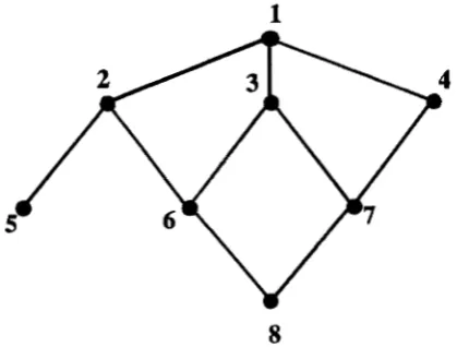
Individual 1 is a noninbred dam that produces the gynogenetic sibs 2, 3 and 4. Individual 5 is a gynogenetically produced clone of 2. Individuals 6 and

7

are referred to as f i ' s

while 8 is referred to as an K2. The genotypes of 5, 6 and

7

cause singularity of A, so their genotypes are not included in the vector u; however their observations are in y, X and Z. For this family, A" and Z are as follows:

1

8

FIGURE 1.-Gynogenetic family structure with dam ( l ) , gynogenetic sibs

(2,

3, 4), clone (5), Fl's ( 6 ,

7 )

and an F2 (8).

and A is singular. However, because individuals 2 and 5 are genetically identical, the observation on individual 5 is a repeated observation on the genotype of individual 2. This information can be accommodated by modifymg the incidence matrix Z and the vector of breeding values u (KENNEDY and SCHAEFFER 1990).

As

a result of this modification, u contains breeding values only for unique genotypes and Z contains a column for each unique genotype. Regarding clones as repeated observations solves the problem of singularity in this case.

Individuals 6 and

7

(Figure 1) are offspring of fully inbred parents, which entails 666 and

S7,

being zero. As a conse- quence, the genotypes of 6 and 7 are identical and equal to the parental average. Because only unique genotypes are included in A", the genotypes of individuals 6 and

7

do not appear in u. However, observations on 6 and 7 provide information on the parental additive genetic effects, which can be incorporated in Z by assigning half of the observation of 6 and

7

to the one parent, and the other half to the other parent. This can easily be done by adding ' / e to the Z matrix at the positions corresponding to the parents of 6 and 7. This generates off-diagonal elements in Z'Z.

Individual 8 (Figure 1) causes problems, because its parents do not directly correspond with a single unique genotype. In %, only contributions of unique genotypes are included. The unique genotypes contributing to the genotype of individual 8 are the grandparents 2, 3 and 4, which contribute, respectively, 1/4, '/e and of the genetic material. Using these

values, (5) can be used to obtain A". Consider an individual

i having fully inbred grandparents j , k, 1 and m, where j and

k are the paternal grandparents and 1 and rn are the maternal grandparents. In s, the contribution of each grandparent is

represented and (5) reduces to adding the following contributions to A":

6"

to element (x, y ) w i t h x = j , m a n d y = j , r n

to element ( i , x) and (x, i) with x = j , m

6'&

to diagonal element ( i , i )

where

The elements 4 . k and u ~ , ~ are elements of A and can be ob-

tained from (6). In fact, those elements indicate the degree of inbreeding in the sire and dam of i and therefore the amount of Mendelian sampling variance in the production of the ith genotype.

4 -1 -1 -1 0

-1 1%

%

I/,

-1

-1 1%

k

71,

-1

-1 -2 -1

z=l

0 0 0 1 0

0 1 0 0 0 '

0 % % 0 0

Using these matrices, and a variance ratio a equal to one, results in the following mixed model equations:

- 8 1 2% 2 1% 1

1 5 -1 -1 -1 0

2% -1 3%

2 %

-1

2 -1

::

_3%

::

-2

1% -1

y4

::

2% -1

- 1 0 -1 -2 -1 5

Solutions for the mixed model equations are as follows:

P

= 14.36, u' = [O.OO 0.26 -0.32 -0.57 -0.061. Additive genetic effects (ebu) for individuals 5, 6 and 7 can be calculated as Zu, resulting in ebu5 = 0.26, ebu, = '/,(0.26 - 0.32), rbv, =

Summarizing, the inverse of the numerator relationship matrix for all possible relationships can be built according to (5). Equation 5 requires the calculation of inbreeding coefficients of all animals, which can be obtained from (6). In (5), the s vector represents the proportion of genes contributed by each unique genotype. Only unique genotypes should be included in u and A". Genotypes that are not unique can be identified by calculating 6,,, with a value of zero indicating that the genotype is not unique.

Optimum designs for estimating heritability: Gynogenesis

opens ways to new experimental drsigns for estimating variance components that can capitalize on the closer relationships between individuals. To investigate the potential value of this technique, optimum gynogenetic sib family sizes for estimating heritabilities and standard errors of heritability estimates will be derived. Optimum design refers to the design that shows the lowest standard error of the estimated heritability. The results will be compared to results for conventional full-sib designs, because both gynogenetic and conventional full-sib designs are subject to effects of common environment and to maternal effects. For a population consisting of N

(4)

1246 P. Bijma, J. A. M. Van Arendonk and H. Bovenhuis

families of n individuals each, the optimum n will be derived, keeping the total number of animals T = Nn constant. Results from a deterministic derivation as well as from stochastic simulation using Gibbs sampling will be shown.

Deterministic approach: The optimum family size depends on the sampling variance of the intraclass correlation t between the members of a family:

V(i)

= 2[1

+

( n - l ) t l ' ( l - t ) ' / ( n - l ) ( T - n ) (9)

(FIS(:HER 1941). When Tis constant and large, V ( i ) as a func- tion of n has a minimum for n = 1

+

l / t . Substituting this result in (9) leads to the following approximation of the sampling variance in the optimum design:

V ( i )

=

8t(l - t)2/T, (10)

which is the same result as obtained by ROBERTSON (1959). Ignoring common environment and maternal effects, the intraclass correlation t between full-sibs equals twice the coefficient of coancestry ( f ) times the heritability: t = 2jh2 = 0.5h2. Optimum family sizes for a conventional full-sib design and the corresponding sampling variance of

h"

are

n = 1

+

2/h', (11)

V(2')

=

16h"(l - %h')'/T. (12)

In a population consisting of gynogenetic sib families, the intraclass correlation is calculated as t = cov(P,, f $ ) / o , , , ~ , ~ ,

where PI and R2 are the phenotypes of two gynogenetic sibs. Ignoring common environment and maternal effects, this results i n

t = %hi, = h'/(hZ

+

l ) , (13)

where his is the heritability in the gynogenetic sib population and h' is the heritability in the noninbred dam population. This result corresponds to t = Zjhi,, ie., twice the coancestry times the heritability. We further wish to estimate h2 and its standard error. Combining (13) and n = 1

+

l / t , the optimum family size for a gynogenetic sib design is

n = 2

+

l/h'. (14)

To obtain the sampling variance of the estimated heritability for a gynogenetic design, the nonlinear relation between t

and h" in (13) is approximated by a linear relation, using a first order Taylor approximation (e.g., ENGLEFIELD 1989). This means that in (13) the relation between t and hZ is approximated by the tangent of the curve in the point of the estimate. The variance is then proportional to the quadratic of the slope of the tangent ( d t / d h ' ) . This results in V ( t ) =

V ( h 2 ) / ( / ?

+

I)', which, when substituted into

(lo),

leads to

V ( &

=

Sh'(h"

+

l ) / T . (15) The relative superiority of the gynogenetic design depends only on the heritability, because sampling variances in both (12) and (15) are inversely proportional to the total number

of animals T.

Stochastic approach: T o validate the deterministic theory, data from 1024 individuals were simulated under a gynogenetic sib design and under a conventional full-sib design with varying family size. The number of families for each design was calculated as N = 1024/n, where n is the family size. N

was rounded to the nearest integer, so the total number of animals can show minor deviations from 1024. Simulated heritability and phenotypic variance were 0.4 and 100. Additive genetic values for sires and dams were chosen from N ( 0 ,

of); additive genetic values for gynogenetic offspring from

N(u,,, of); additive genetic values for full-sibs from N( ' / y u ,

+

'/.u,,, %a:,); and phenotypic values for the zth individual from

2

1.8

1.6

1.4

1 .z

1

0.8

0.6

0.4

o.2 0

?

0.1 0.2 0.3 0.4 0.5 0.6 0.7 0.8 0.9 1

h'

FIGURE 2.-Standard error of

x'

for an optimum gynogenetic design relative to an optimum conventional full-sib design, for different true heritabilities.

N ( p

+

u,, a:), where N denotes the normal distribution, at

is the additive genetic variance in the parental population, 0: is the non-genetic variance, u,, ud and u, are the additive genetic value for sire, dam and individual, and ,LL is the popula-

tion mean. For each situation, 25 replicates were performed, except for the designs close to the deterministically determined optimum design, for which 7 5 replicates were performed.

Bayesian inferences on variance components were made using a Gibbs sampling algorithm. The model was

y = ? @ + Z u + e . (16)

As fixed effect, only a general mean was included. For the conventional full-sib design, marginal posterior distributions were generated using the Gibbs sampling program maGGic developed by JANsS et al. (1995). For the gynogenetic sib design, the procedure is described in the APPENDIX. Flat prior distributions for variance components were used for both designs. For both the gynogenetic and the full-sib design, posterior distributions were based on a single chain of 40,000 Sam- ples for each replicate. Starting values for the variance

components were equal to the simulated values.

The obtained Gibbs chain was thinned according to the approach suggested by RZFEIUY and LEwls (1992). From the obtained posterior distribution, the mode was used as an estimate of the parameter ( i e . , variance component) and the posterior standard deviation was used as the equivalent of the standard error of the parameter estimate.

RESULTS

Deterministic approach: Using (14) and

(1

1

), opti- m u m family sizes f o r a heritability of 0.4 are 4.5

for

a

gynogenetic sib design and 6.0 for a conventional full- sib design. For a total of 1024 animals, the standard errors of are

0.066

a n d 0.063, respectively. In Figure

2,

the standard error of the estimated heritability for

an optimum gynogenetic sib design relative to an opti- m u m c o n v e n t i o n a l full-sib design is presented for differ- e n t true heritabilities. This figure was obtained using

(5)

Genetic Evaluation With Inbreeding

TABLE

1

Standard deviations of variance component estimates obtained from stochastic simulation

Gynogenetic sib design Full-sib design

N*n No. repl stda: stday" stda: stda:',*" N*n No. repl stdaj stda'f*" stdu:', stday"

16*64 25 18.8 12.3 18.0 12.0 16*64 25 10.8 7.5 19.3 12.5

64*16 25 10.1 9.8 9.0 6.7 64*16 25 6.6 7.2 10.5 8.7

128*8 25 8.8 9.2 7.1 5.7 128*8 25 5.9 5.9 8.2 6.7

146*7 25 8.6 10.4 6.6 7.3 146*7 75 5.9 5.7 7.9 7.1

171*6 75 8.6 8.5 6.4 5.6 171*6 75 6.0 5.9 7.7 7.6

256*4 75 8.8 9.4 6.0 5.6 256*4 25 6.3 7.8 7.4 8.5

341*3 25 9.2 10.5 6.1 5.6 341*3 25 6.9 7.4 8.1 8.5

205*5 75 8.4 9.1 6.1 5.5 205*5 75 6.1 6.0 7.7 6.5

No. repl, number of replicates; stda;, posterior standard deviation of a: averaged over replicates; stday, standard deviation

'' Calculated as follows: (x, - x,,d

'/

(No. repl - 1) , where x, is the mode of the posterior distribution for the ith replicate between the modes of replicates for a:. Simulated heritability and phenotypic variance: h2 = 0.40, ai = 100.

and x,'~,~ is the mode averaged over all replicates for this design.

gynogenetic sib design and for the conventional full- sib design have equal standard errors. From

(11)

and (14) it follows that the optimum family size is always smaller for a gynogenetic design. At low values of h2,

the optimum full-sib family size is approximately twice the optimum gynogenetic sib family size. When h' approaches unity, the optimum family size for both designs approaches three.

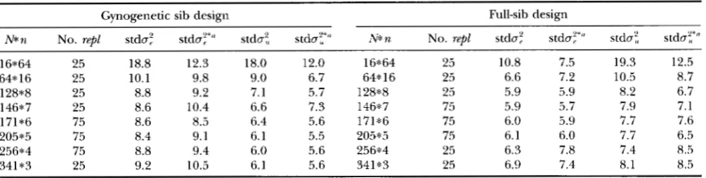
Stochastic approach Posterior standard deviations of the variance components obtained from stochastic simulation are presented in Table

1

for both designs. Besides the posterior standard deviations, the standard deviations between the modes of replicates are also in Table

1

(indicated by an asterisk). It can be seen, that for large family sizes the standard deviation between the modes of replicates ( s t & ; * ) is smaller than the posterior standard deviation averaged over replicates

( 5 t h : ) . When the family sizes are smaller and the esti-

mates become more accurate, this difference disap- pears. For gynogenetic designs, 0: is estimated more accurately than

03,

whereas for full-sib designs this relation is reversed (see Table

1).

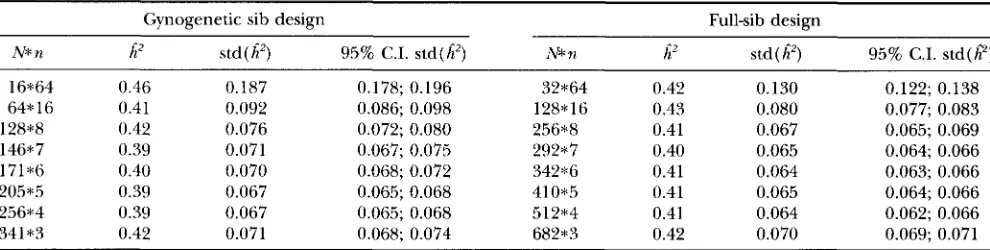
Modes and standard deviations of estimated heritabilities averaged over replicates are presented in Table

2

together with 95% confidence intervals for the standard deviations of the estimated heritability. For both designs, standard deviations of the heritability estimates rapidly decreased when family size was lowered from 64 to eight family members by increasing the number of families. The optimum family size for a gynogenetic design was around four to five family members. For the full-sib design, the optimum family size could not be determined very precisely from the confidence intervals, but was around five to six family members. These results are in agreement with the deterministically determined optimum family sizes. Standard errors for the optimum design obtained from the deterministic derivation were 0.066 for a gynogenetic design and 0.063 for a conventional full-sib design. Those standard errors

are within the confidence intervals for the standard deviations presented in Table

2.

For a heritability of 0.4, no significant difference in accuracy of the estimated heritability between a gynogenetic and a full-sib design could be found from simulation, as was to be expected from Figure

2.

DISCUSSION

Under gynogenetic reproduction, the additive genetic variance in the offspring population is doubled compared to the noninbred dam population and is equally distributed within and between gynogenetic sib families

(BONGEFS

et ul. 1996). A method for breeding value estimation for gynogenetic families using mixed model equations is presented. In the mixed model equations, the inverse of the numerator relationship matrix

A

is required. A general method for creating this inverse is presented. As a result, A" can be built for any population that has unusual relationships. For the use of this method, the diagonal elements of A are required, which means that the inbreeding coefficients of individuals have to be calculated. Identical genotypes can be produced using gynogenesis. These identical genotypes cause singularity of the

A matrix. However,

observations on individuals having identical genotypes can be regarded as repeated observations on the same genotype, which can be accommodated by considering only the unique genotypes.

(6)

P. Bijma, J. A. M. Van Arendonk and H. Bovenhuis

TABLE 2

Estimated heritabilities

Gynogenetic sib design Full-sib design

N* n h 2 std (

A')

95% C.I. std(6') N* n

A'

std ( /?) 95% C.I. std(ff)

16*64 0.46 0.187 0.178; 0.196 32*64 0.42 0.130 0.122; 0.138

64* 16 0.41 0.092 0.086; 0.098 128*16 0.43 0.080 0.077; 0.083

146*7 0.39 0.071 0.067; 0.075 292*7 0.40 0.065 0.064; 0.066

128*8 0.42 0.076 0.072; 0.080 256*8 0.41 0.067 0.065; 0.069

171% 0.40 0.070 0.068; 0.072 34'2*6 0.41 0.064 0.063; 0.066

205*5 0.39 0.067 0.065; 0.068 410*5 0.41 0.065 0.064; 0.066

256*4 0.39 0.067 0.065; 0.068 512*4 0.41 0.064 0.062; 0.066

341*3 0.42 0.071 0.068; 0.074 682*3 0.42 0.070 0.069; 0.071

h',

mode of heritability estimates averaged over replicates; std(/?), standard deviation of heritability estimates averaged over replicates; 95% C.I., 95% confidence interval. Simulated heritability and phenotypic variance: h2 = 0.40, 0; = 100.

bred and can be represented by a single genotype. The

Fl

generations can be represented as the average of the founder lines, Le., not unique. Individuals in subse- quent generations have unique genotypes. The approach presented in this paper can be utilized to ana- lyze data of such experiments and accommodates completely inbred founder lines.

Optimum family sizes for estimating heritabilities were found to be smaller for gynogenetic sib families than for conventional full-sib families. Compared to the biological capacity of fish, optimum family sizes are very small. Only for heritabilities below 0.35, there is a small advantage in accuracy of the estimated heritability for gynogenetic sib families. For higher heritabilities, there is a clear disadvantage.

Clone lines enable the measurement of different traits on the same genotype, for example, carcass quality at different ages. Clone lines might therefore be very useful for estimating the genetic correlations. Clone lines can also be useful for estimating genotype by environment interaction, because performance on the same genotype can be observed in different environments.

Because of the increased heritability and the doubled additive genetic variance in the offspring population, gynogenetic reproduction can be useful for selection purposes. However, inbred individuals show inbreeding depression. Furthermore, the phenotypic variance may increase due to embryonic damage

(BONGERS

et al.

1996) or due to an increased sensitivity of inbred individuals to environmental influences (FALCONER 1989). For these reasons, the increase in heritability can be lower than theoretically expected.

Cloning by means of gynogenesis offers the opportu- nity to capitalize on nonadditive genetic effects. It seems promising to produce crossbred clones to make optimum use of nonadditive effects. This can be done by using gynogenetically produced individuals from different lines as parents. In this way the additive genetic superiority of selected gynogenetic individuals can be combined with the effect of heterosis.

A

method to

estimate genetic values for selection of parents as developed here, is crucial in such schemes. Among these crossbreds there is no genetic variation, which would promote product uniformity.

We thank JACK C. M. DEKKERS for carefully reading this paper and giving useful comments. In addition we thank HANS KOMEN and GUUS B. J. BONGEKS for introducing us into the world of gynogenesis.

LITERATURE CITED

BONGERS, A. B. J., H. BOVENHUIS, A. C. VAN STOKKUM, G. F. WIECER- TIES, B. ZANDIEH-DOUMI et al. 1996 Distribution of genetic variance in gynogenetic and androgenetic families. Aquaculture

(in press).

ENGI.EFIEI.U, M.J., 1989 Mathematical Methods for Engznem'ng and Sci- Pnce Students. Edward Arnold, London.

FALCONER, D. S., 1989 Introduction to Quantitative Genetics. Longman Group Ltd., Essex, UK.

FISCHER, R. A,, 1941 Statistical Methods for Research Workers. Oliver &

Boyd, Edinburgh, UK.

HENDERSON, C. R., 1976 Asimple method for computing the inverse of a numerator relationship matrix used in prediction of breeding values. Biometrics 32: 69-83.

JANSS, 1,. L. G., R. THOMPSON andJ. A. M. VANARENDONK, 1995 Appli- cation of Gibbs sampling for inference in a mixed major gene- polygenic inheritance model in animal populations. Theor. Appl. Genet. 91: 1137-1147.

KENNEDY, B. W., and J. E. MOXLEY, 1975 Comparison of genetic group and relationship methods for mixed model sire evaluation.

J. Dairy Sci. 58: 1507-1514.

KKNNEDY, B. W., and L. R. SCHAEFFER, 1990 Reproductive technol- ogy and genetic evalaution, pp. 507-532 in Advances in Statistical Methods f i r Genetic Improvement of Livestock, edited by D. GIANOIA and K. HAMMOND. Springer-Verlag, Berlin.

KOMEN, J , , A. B. J. BONGERS, C. J. J. RICHTER, W. B. VAN MUISWINKEL. and E. A. HUISMAN, 1991 Gynogenesis in common carp

(cy@'-

nu.\ carpio I.. ) 11: The production of homozygous gynogenetic clones and F1 hybrids. Aquaculture 92: 127-142.

LAIDLAW, H. H., and R. E. PAGE, 1986 Mating designs. pp. 323-344 in Bee Genetics and Breeding, edited by T. E. RINDERER. Academic Press, New York.

MEYFR, K., 1989 Estimation of genetic parameters, pp. 161-167 in

Evolution and Animal Breeding, edited by G. W. HIIS. and T. F. C.

MACKAY. CAB International, Wallingford,; UK.

QLI.US, R. L., 1976 Computing the diagonal elements and inverse

of a large numerator relationship matrix. Biometrics 32: 949-

RAFEKD, A. E., and S . M. LEWIS, 1992 How many iterates in the 953.

Gibbs sampler?, pp. 765-776 in Bayesian Statistics, edited by J. M.

(7)

1249

ROBERTSON, A., 1959 Experimental design in the evaluation of genetic parameters. Biometrics 15: 219-226.

SMITH, S. P., and F. R. AXLAIRE, 1985 Efficient selection rules to

increase non-linear merit: application to mate selection. Genet.

Sel. Evol. 17: 387-406.

VAN ARENDONK, J. A. M., B. TIER and B. P. KINGHORN, 1994 Use

of multiple genetic markers in prediction of breeding values. Genetics 137: 319-329.

WAN(;, C. S., J. J. RUTLEDCE and D. GIANOIA, 1994 Bayesian analysis of mixed linear models via Gibbs sampling with an application to litter size in Inberian pigs. Genet. Sel. Evol. 26: 91-115.

Communicating editor: M. K. UENOYAMA

APPENDIX

Bayesian analyses

implemented via

Gibbs sam-

pling:

In each cycle of Gibbs sampling, a sequence of realizations was computed conditional on the data and on the realizations of the previous cycle. Realizations for the tth cycle were sampled in the order

P''',

u['],

realizations were similar to JANSS et al.

(1995).

For illus- tration purposes, the conditional distributions are shown in Equation

A2

for all unique genotypes in the family structure of Figure

1.

In the analyses to deter- mine the optimum family size, however, only dams and gynogenetic sibs were included and contributions from other kinds of individuals were omitted from their conditional equations. In Figure

1,

different types of individuals can be distinguished. Individual

1

is referred to as a dam, individuals

2-4

are referred to as gynogenetic sibs, 6 and

7

are referred to as f i ' s , and individual

8

is referred to as an

F2. The genotypes of the individuals

5-7

are not included in u because these genotypes are not unique. Notation is similar toJANss et al.

(1995).

As

first step in a cycle of Gibbs sampling, the general mean was sampled as

a2 ,I

,

a:"].

Conditional distributions used to sample the

Sample /3['+11 from

N ( j / n , ,

c ~ ? " ~ / n , ) ,

( A l )

where

N

denotes the normal distribution; f is the sum of all elements in jr =

y

- ZU"];

a

:

[

'

]

is the realization of the nongenetic variance from the previous cycle; and n,

is the total number of observations.

So

the fixed effect is sampled conditional on the realized genetic effects and on the non-genetic variance from the previous cycle.

Genetic effects were sampled starting with the earliest generation. The additive genetic effect of genotype i

was updated as:

Sample u:'+~' from N ( c j / d j , a ; [ " / d , ) ,

(A2)

where dtu, = c, are the mixed model equations for the ith individual. Elements in

(A2)

are as follows.

For the dams:

c, = jz

+

aZk6kkuF1, d, =

1 +

a(b2'

+

&Skk),

where

Yi

is the ith element of

jr

=

(y

-

m't+ll);

k indicates each gynogenetic sib descending from dam i;

a

is the variance ratio aS/a:; and

6'

is the reciprocal of the Mendelian sampling term, as described in the mixed model section.

For the gynogenetic sibs:

ci =

j ;

+

a6'*U6t+*] - a ~ k 6 k k S k , i ~ @ d ~ , @ r u @ , y 1 . 1

- % C , u ; ' ]

+

aCkSk,ldkkUb'I

d, =

a,,

+

a

(6"

+

Ck$,,dkk),

where i is the gynogenetic sib; d is the dam of i; k

refers to an F2; gpr refers to the grandparents of the F2, excluding

i

itself;

p

refers to the mates of i for the production of

Fl's;

and a,, in the ith diagonal element of the Z'Z matrix. The element s ~ , ~ is the ith element of the s vector for individual k, and indicates the contribution of i to the genotype of k. The same holds for sk,@. For instance, for the family structure in Figure

1,

= 1/4, and = When it is unclear whether a

genetic effect used is from state t or

t

+

1,

the state is not specified.

For the F2:

c, =

j t

+

a 6 ' z C @ ~ 8 , r l , r u ~ l l , d, =

1 +

abz2,

where C , g S , , , u g 1 ] indicates summation of the genetic effects over all grandparental genotypes contributing to

i,

weighted by their contribution.

Residual and genetic variances were sampled from inverted chi-squared distributions. Those variance components were updated as follows:

sample ag"+ll from ere/X:lzt-2),

(A31

sample a:['+'] from

u'['+~~A-'u['~'~/x~~,-~),

(A4)

where e =

(y

-

X p [ ' + ' ]

- Z u r t + l l ) ;

A is the numerator

relationship matrix; and are random devi- ates from chi-squared distributions with ( n , -

2 ) and

( q

-

2)

degrees of freedom;

n,

is the number of observations; and

q

is the number of genotypes. Degrees of freedom ( n , -

2)

and

( q

-

2)

indicate a flat prior for variance components

(WANG

et al.

1994). A

scalar computation of the quadratic urA"u is

C j G

+

Cp.(

ui -

1/2ud

- where indices d and s indicate dam and sire o f j

(QUAAS

1976).

The first summation is over all base genotypes and the second over all nonbase genotypes. For the gynogenetic sibs, the second summation is modified to C,Gu(u, -

ud)',

and for the

E2's

to