Aging comets and their meteor showers

Western University Western University

Scholarship@Western

Scholarship@Western

Electronic Thesis and Dissertation Repository

7-28-2016 12:00 AM

Aging comets and their meteor showers

Aging comets and their meteor showers

Quanzhi Ye

The University of Western Ontario

Supervisor Peter Brown

The University of Western Ontario Graduate Program in Astronomy

A thesis submitted in partial fulfillment of the requirements for the degree in Doctor of Philosophy

© Quanzhi Ye 2016

Follow this and additional works at: https://ir.lib.uwo.ca/etd

Part of the The Sun and the Solar System Commons

Recommended Citation Recommended Citation

Ye, Quanzhi, "Aging comets and their meteor showers" (2016). Electronic Thesis and Dissertation Repository. 3903.

https://ir.lib.uwo.ca/etd/3903

This Dissertation/Thesis is brought to you for free and open access by Scholarship@Western. It has been accepted for inclusion in Electronic Thesis and Dissertation Repository by an authorized administrator of

Comets are thought to be responsible for the terrestrial accretion of water and organic mate-rials. Comets evolve very quickly, and will generally deplete their volatiles in a few hundred revolutions. This process, or the aging of comets, is one of the most critical yet poorly un-derstood problems in planetary astronomy. The goal of this thesis is to better understand this problem by examining different parts of the cometary aging spectrum of Jupiter-family comets (JFCs), a group of comets that dominates the cometary influx in the near-Earth space, using both telescopic and meteor observations.

We examine two representative JFCs and the population of dormant comets. At the younger end of the aging spectrum, we examine a moderately active JFC, 15P/Finlay, and review the puzzle of the non-detection of the associated Finlayid meteor shower. We find that, although having been behaving like a dying comet in the past several 102 _{years, 15P/Finlay have}

pro-duced energetic cometary outbursts without a clear reason. Towards the more aged end of the spectrum, we examine a weakly active JFC, 209P/LINEAR. By bridging telescopic observa-tions at visible and infrared wavelength, meteor observaobserva-tions and dynamical investigaobserva-tions, we find that 209P/LINEAR is indeed likely an aged yet long-lived comet. At the other end of the

spectrum, we examine the population of dormant near-Earth comets, by conducting a compre-hensive meteor-based survey looking for dormant comets that have recently been active. We find the lower limit of the dormant comet fraction in the near-Earth object (NEO) population

to be 2.0_±1.7%. This number is at the lower end of the numbers found using dynamical and

telescopic techniques, which may imply that a significant fraction of comets in the true JFC population are weakly active and are not yet detected.

These results have revealed interesting diversity in dying or dead comets, both in their behavior as well as their nature. An immediate quest in the understanding of cometary aging would be to examine a large number of dying or dead comets and understand their general characteristics.

Keywords:asteroid, comet, meteor, meteoroid

Co-Authorship Statement

This thesis dissertation is based on several published or submitted manuscripts which are listed as follows:

• Chapter 2: Bangs and Meteors from the Quiet Comet 15P/Finlay, published in the As-trophysical Journal (2015), Volume 814, Number 1, with the authors being Quan-Zhi Ye, Peter G. Brown, Charles Bell, Xing Gao, Martin Maˇsek, and Man-To Hui. The contri-bution of each coauthor is: Peter Brown provided extensive advice and suggestions to improve the manuscript; Charles Bell, Xing Gao and Martin Maˇsek operated the tele-scopes at Vickburg, Xingming Observatory and Pierre Auger Observatory and provided the data; Man-To Hui helped with the preliminary reduction of the data from Xingming Observatory.

• Chapter 3: When comets get old: A synthesis of comet and meteor observations of the low activity comet 209P/LINEAR, published in Icarus (2016), Volume 264, p. 48–

61, with the authors being Quan-Zhi Ye, Man-To Hui, Peter G. Brown, Margaret D. Campbell-Brown, Petr Pokorn´y, Paul A. Wiegert, and Xing Gao. The contribution of each coauthor is: Man-To Hui provided extensive suggestions on the development of the dust model; Peter Brown and Paul Wiegert provided extensive suggestions and reviews of the manuscript; Margaret Campbell-Brown provided the meteor ablation code; Petr Pokorn´y helped with the determination of the mass indices of the meteor shower; Xing Gao operated the telescope at Xingming Observatory and provided the data.

• Chapter 4: Dormant Comets Among the Near-Earth Object Population: A Meteor-Based Survey, in press at the Monthly Notices of the Royal Astronomical Society, with

the authors being Quan-Zhi Ye, Peter G. Brown and Petr Pokorn´y. Peter Brown and Petr Pokorn´y provided extensive suggestions and reviews of the manuscript.

As the author of this thesis and the lead author of these papers, I initiated the original

the telescopic and meteor data. However, it is only fair to point out that my supervisor, Pe-ter Brown, provided extensive guidance, suggestions and comments throughout my research. All radar meteor observations presented in this thesis were obtained by the Canadian Meteor Orbit Radar (CMOR), developed and maintained by the Western Meteor Physics Group at the University of Western Ontario.

Acknowledgments

First and foremost, I thank my advisor, Peter Brown, for all his guidance and support that help me reach my potential as a scientist. As a stargazer at heart I consider myself extremely fortunate to be able to work with a great mind who is both passionate and knowledgeable. I am constantly amazed by his ability to convoy a difficult concept in a straight and lighthearted way.

I thank my advisory committee, Margaret Campbell-Brown and Paul Wiegert, for their support and for many helpful discussions that took place on or off their duty. For countless times they (together with Peter) encouraged me to bravely take the challenges and be better.

Thanks to all the members of the Western Meteor Physics Group, as well as to the stu-dents, postdocs, staffs and faculties at the Department of Physics and Astronomy, who helped me progress and made my time at Western enjoyable. I couldn’t possibly acknowledge ev-eryone here, but the following people deserve special mention: Abedin Abedin, Pubuditha Abeyasinghe, Sayantan Auddy, Sebasti´an Bruzzone, Pauline Barmby, Clara Buma, David Clark, Tushar Das, Jason Gill, Jodi Guthrie, Renjie Hou, Bushra Hussain, Mahdia Ibrahim, Sina Kazemian, Shayamila Mahagammulla, Stanimir Metchev, Petr Pokorn´y, Fereshteh Ra-jabi, Sahar Rahmani, Edward Stokan, Dilini Subasinghe, Robert Sica, Aaron Sigut, Maryam Tabeshian, and Robert Weryk. Thanks also to all my badminton and table tennis buddies, whom I had a lot of fun with.

Thanks to the many amateur and professional astronomers, who inspired and helped me over the years I love and study astronomy. These include Eric Christensen, Xing Gao, Alan Harris, Song Huang, Man-To Hui, Matthew Knight, Jian-Yang Li, Chi Sheng Lin, Hung-Chin Lin, Robert Matson, Robert McNaught, Nalin Samarasinha, Liaoshan Shi, Tim Spahr, Jin Zhu, and many others.

Thanks to all the great composers, notably Bach, Beethoven, Schubert, Dvoˇv´ak and Sibelius, for writing the great music and lighting up us followers. For many times their great sounds

me part of the music, either as audience or player.

Thanks to my parents and other family members for love, encouragement and support, no matter how far I have had been away from my dreams. Special thanks to my uncle, H.S., for all his fun stories and tips on how to become a scientist.

I wish to commemorate my grandmother, C.Y., and grandfather, K.G. They shall be very happy to see me at where I am today.

Finally, thanks to my wife, Summer, for all the great conversations and memories, for making andfinding delicious meals/eateries, and for being with me at all the glorious triumphs and bluest moments.

To the Great Inhabitants of H.C.

Certificate of Examination ii

Abstract iii

Co-Authorship Statement iv

List of Figures xiii

List of Tables xxiii

List of Appendices xxvi

List of Abbreviations and Symbols xxvii

1 Introduction 1

1.1 Basics . . . 1

1.2 History of Comet and Meteor Studies . . . 7

1.3 Evolution of Comets and Their Meteoroid Streams . . . 11

1.3.1 Repositories of Comets . . . 11

1.3.2 End States of Comets . . . 14

1.3.3 Formation and Evolution of Meteoroid Streams . . . 15

1.4 Observations of Comets and Meteors . . . 16

1.4.1 Observation of Comets . . . 16

1.4.2 Observation of Meteors . . . 18

1.4.3 Modeling of Cometary Dust and Meteoroids . . . 20

1.4.4 Meteoroid Stream Identification and Stream-Parent Linkage . . . 22

1.5 Previous Studies . . . 24

1.5.1 Studies of Weakly-Active and Dormant Comets . . . 24

1.5.2 Meteor Studies . . . 27

1.6 Questions for This Thesis . . . 29

2 Moderately active comet: the case of 15P/Finlay 37 2.1 Introduction . . . 37

2.2 Observations . . . 40

2.2.1 Amalgamation of Outburst Reports . . . 40

2.2.2 Observation and Image Processing . . . 43

2.3 Analysis . . . 44

2.3.1 General Morphology and Evolution of the Outbursts . . . 44

2.3.2 Dust Model and Kinematics of the Ejecta . . . 45

2.4 Discussion . . . 50

2.4.1 Nature of the Outburst . . . 50

2.4.2 The Finlayid Puzzle Revisited . . . 51

2.4.3 The 2021 Earth Encounter of the 2014/2015 Outburst Ejecta . . . 54

2.5 Summary . . . 56

3 Weakly active comet: the case of 209P/LINEAR 61 3.1 Introduction . . . 61

3.2 The Comet . . . 64

3.2.1 Observation . . . 64

3.2.2 Results and Analysis . . . 65

Start of Cometary Activity and General Morphology . . . 65

Modeling the Dust . . . 67

3.3 The Meteors . . . 75

3.3.1 Instrument and Data Acquisition . . . 75

3.3.2 Results and Analysis of the 2014 Outburst . . . 77

General Characteristics . . . 77

Meteoroid Properties . . . 81

3.3.3 Camelopardalid Activity in Other Years . . . 83

3.3.4 Modeling the Dust (II) . . . 84

3.4 Discussion . . . 89

3.4.1 The Dynamical Evolution of 209P/LINEAR . . . 89

3.4.2 Nature of 209P/LINEAR and Comparison with Other Low Activity Comets . . . 94

3.5 Conclusions and Summary . . . 95

4 Dormant comets: a meteor-based survey 104 4.1 Introduction . . . 104

4.2 Identification of Potential Shower-Producing Objects . . . 107

4.2.1 Dormant Comets in the NEO Population . . . 107

4.2.2 Objects with Detectable Meteor Showers . . . 107

4.3 Prediction of Virtual Meteor Showers . . . 113

4.4 Observational Survey of Virtual Meteor Activity . . . 116

4.5 Results and Discussion . . . 117

4.5.1 Annual Showers from Old Streams . . . 117

4.5.2 Outbursts from Young Trails . . . 124

4.5.3 Discussion . . . 127

4.6 Conclusion . . . 131

5 Conclusions 157

A Details of the Cometary Dust and Meteoroid Stream Model 162

B CMOR Basics 169

B.1 The CMOR System . . . 169

B.2 Echo Types . . . 172

B.3 Orbit Determination . . . 174

B.4 Wavelet Analysis . . . 175

C Copyright Permissions 178

Curriculum Vitae 187

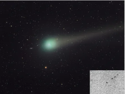
1.1 Morphological evolution of comet C/2007 N3 (Lulin). Lower-right: Comet Lulin (center dot) at the time it was discovered by the author and Chi Sheng Lin (2007 July 11; rh = 6.4 AU), credit: Lulin Observatory/National

Cen-tral University. Full image: Comet Lulin near perihelion (2009 February 28; rh = 1.4 AU), taken by Johannes Schedler (Panther Observatory), used with

permission. . . 3

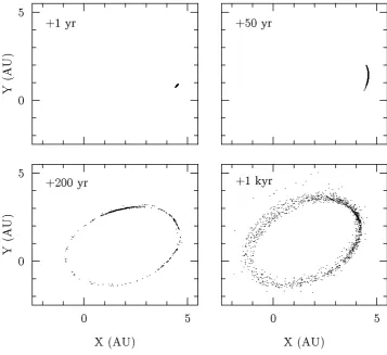
1.2 Evolution from meteoroid trail into stream: meteoroid ejection from comet 209P/LINEAR after 1 (a short arc of meteoroid trail), 50 (a longer arc of me-teoroid trail), 200 (spread to the entire orbit) and 1000 years (a more spread, dispersed stream). Meteoroids drift away from their initial position on the orbit due to ejection velocity as well as differential perturbation. . . 4

1.3 Elements that define an orbit: perihelion distanceq, semimajor axisa(note that for clarity, the quantity of 2a is shown in the figure), longitude of ascending

node Ω, and argument of perihelion ω. The eccentricity e is not explicitly

shown, but can be derived through the relation q = a(1−e). The symbol of

Υstands for the First Point of Aries. The horizontal plane is the ecliptic plane (the orbital plane of the Earth) and the central red point is the Sun. . . 5

1.4 Depiction of the Kuiper belt (insetfigure) and the Oort cloud in the Solar Sys-tem. Rendered by William Crochot (JPL). . . 11

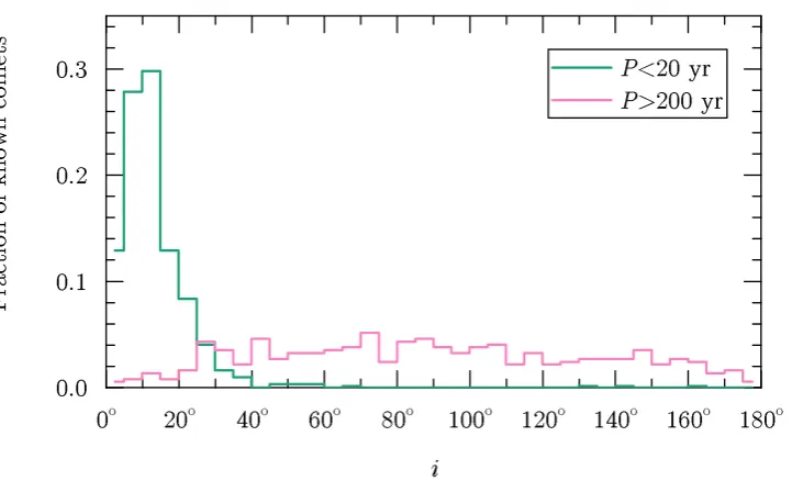
1.5 Distribution of orbit inclination of SPCs withP < 20 yr and LPCs withP >

200 yr, based on data extracted from the JPL Small-Body Database (retrieved 2016 June 16). It is clear that most SPCs stay close to the ecliptic plane while the distribution of LPCs orbits is largely isotropic. . . 12

1.6 Definition of LPCs, HTCs, Damocloids, JFCs, active and asteroids based on the Tisserand parameter (TJ). Definition adapted from Levison (1996) and Jewitt

et al. (2015). . . 13

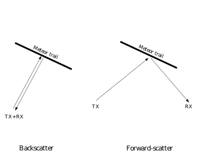
1.7 Observing geometry for backscatter (left) and forward-scatter systems. TX stands for transmitter and RX stands for receiver. . . 20

1.8 Syndyne diagram of a comet. Reproduced from Figure 1 of Ye & Wiegert (2014). 21

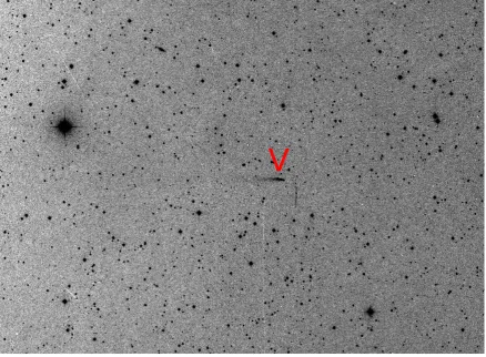
1.9 Comet 107P/(4015) Wilson-Harrington at discovery (1949 November 19). The comet is marked by an arrow. The plate was taken by the 48-inch Oschin Tele-scope at Palomar Observatory appropriated to B-band. The image has been enhanced by the European Southern Observatory (ESO) photographic labora-tory at Garching. . . 26

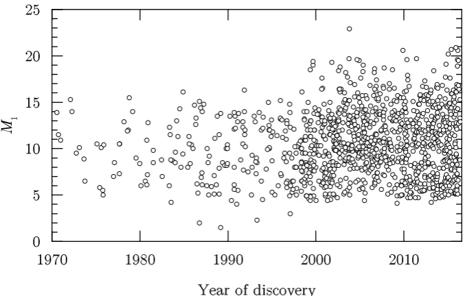
1.10 The distribution of total cometary absolute magnitudes (M1) versus the year

discovered. The magnitude data is retrieved from the JPL Small-Body Database on 2016 June 16. It can be seen that most comets with M1 > 15 were found

after about the year 2000. . . 27

2.1 Nucleus magnitude of 15P/Finlay around the time of (a) thefirst outburst, and (b) the second outburst. The Minor Planet Center (MPC) magnitudes (plotted in crosses) are extracted from the Observations Database on the MPC website. The Xingming magnitudes (plotted in red dots) are derived from the moni-toring observations by the Xingming 0.35-m telescope with aperture radius

ρ = 5000 km. The magnitudes are normalized toΔ = rh = 1 AU assuming a

brightening raten=4 (Everhart, 1967). . . 40

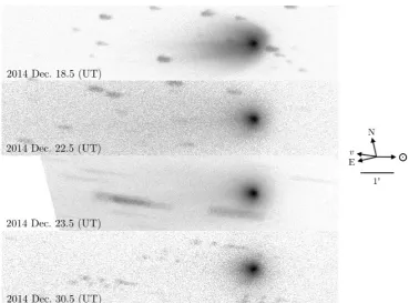
shows the direction to the Sun, the comet’s velocity vector and the directions of the plane of the sky. . . 41

2.3 Composite images of 15P/Finlay images for the second outburst as observed at Xingming Observatory. The images have been stretched in asinh scale. The scale bar shows the direction to the Sun, the comet’s velocity vector and the directions of the plane of the sky. . . 42

2.4 Observed surface brightness profiles (scatter dots) and the best-fit dust models (color lines) for FRAM and Vicksburg observations. The assumed outburst epochs (see main text) are denoted as t1 for the first outburst and t2 for the

second outburst. The regions that are dominated by submicron-sized particles are masked away from the modeling as described in the main text. For the profile on 2015 Jan. 19 an additional region is masked due to contamination from a background star. . . 49

2.5 Dynamical evolution of the perihelion distance of 100 clones of 15P/Finlay in the interval of 1000–2000 A.D. . . 52

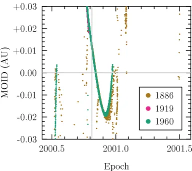
2.6 The distribution of the dust trails released by 15P/Finlay during its 1886, 1909 and 1960 perihelion passages in 2001. Vertical gray line marks the time that the Earth passes the trails. It can be seen that the trails cross the Earth’s orbit, suggestive of the possibility of a direct encounter with the Earth. . . 53

2.7 The variation of the wavelet coefficient at the calculated Finlayid radiantλ₋

λ_� = 66◦,β =−25◦, vG = 13 km·s−1using the stacked “virtual year” CMOR

data. The shaded area is the expected time window for Finlayid activity (solar longitudeλ_{� ∼}193◦). . . 54

2.8 Encounter of 15P/Finlay’s 2014/2015 outburst ejecta in 2021 Oct. 6/7. Sub-figure (a) corresponds to the simulation results assuming the earliest possible

outburst epoch (2014 Dec. 15.4 UT for thefirst outburst, 2015 Jan. 15.5 UT for the second outburst), while (b) corresponds to the results assuming the latest possible outburst epoch (2014 Dec. 16.0 UT for the first outburst, 2015 Jan. 16.0 UT for the second outburst). . . 55

3.1 The 2014 Apr. 9 GMOS-N image (stretched in logarithmic scale) superim-posed with the synchrone model. The ages of the synchrone lines (dashed lines) are (in counterclockwise order) 10, 25, 50 and 100 d respectively. The oldest visible dust was released atτ_∼50 d, appropriate to late Feb. 2014. . . . 65

3.2 Composite images of 209P/LINEAR taken by Xingming 0.35-m telescope and Gemini Flamingo-2 on 2014 May 18 and 25. The images are stretched in asinh scale and are rotated to have north-up east-left. . . 66

3.3 Observed (colored pixels) and modeled (contours) surface brightness profiles for the Xingming image (upper figure) and the Gemini F-2 image (lower fig-ure; the sunward data is shifted downwards for clarity). The surface bright-ness profiles are normalized to the pixel intensity 3 FWHMs behind the nu-cleus along the Sun-comet axis to avoid contamination from the nunu-cleus signal. The mean best model for both the Xingming and the Gemini F-2 images has

βrp,max =0.004 to 0.005,V0=40 m·s−1,q=3.8 andσν =0.3. . . 70 3.4 Representative attempts tofit the sunward section of the coma in the Gemini

F-2 image. The observed and modeled profiles are all normalized to 3 FWHMs away from the nucleus along the comet-Sun axis. These models haveq=−3.8

andβrp,max =0.004. . . 71

dle figure: derived coma+nucleus profile by subtracting the modeled profile from the observed profile. Lowerfigure: nucleus-only profile, derived from subtracting the linear portion of the coma profile. The X-axis corresponds to the Sun-comet axis. . . 73

3.6 Determination of the optimal radiant and velocity apertures. Radiant aperture is centered atλ₋λ_� = 38◦, β = +57◦ in the Sun-centered ecliptic coordinate

system, (in-atmosphere) velocity aperture is centered at vm = 18.8 km·s−1.

Background values are extracted from non-outburst dates ±2 days from the outburst date (i.e. 2014 May 22 and 26). The optimal radiant and speed aper-tures are determined to be 10◦_{and 11% respectively (marked by arrows). The}

velocity aperture is determined for the spatial aperture of 10◦_{. . . 76}

3.7 Top: Variations of the overdense meteor fraction with Poisson errors, binned in 2 h intervals. A dip (i.e. larger proportion of small meteoroids) is appar-ent around the peak hour (7–8h UT). Bottom: Raw numbers of overdense and underdense Camelopardalid meteors detected by CMOR, binned in 15 min in-tervals. . . 78

3.8 Determination of mass indices for the underdense (upperfigure) and overdense (lowerfigure) populations. The mass indices are determined to be 1.84±0.07 for underdense and 2.02_±0.19 for overdense meteors. The dashed lines show

the best fit as determined by the technique developed by (Pokorn´y & Brown 2015, in prep). The uncertainties are based on the distributions of the posterior probabilities obtained by the MultiNest algorithm (Feroz et al., 2013). The correction of echo duration is described in Ye et al. (2013). . . 79

3.9 The variation of the flux (corrected to a limiting magnitude of +6.5) of the 2014 Camelopardalid meteor outburst as observed by CMOR and IMO visual observers. The CMOR observations are binned in 1 hr intervals. Error bars denote Poisson errors. . . 80

3.10 Specular height distribution of the underdense meteor echoes observed by CMOR for the 2011/12 Draconid outbursts (denoted as DRA11 and DRA12) and 2014 Camelopardalid outburst (denoted as CAM14), plotted as shaded bars. Specu-lar height distribution of sporadic meteors (generated using all meteors detected by CMOR withvmwithin 5% from 20 km·s−1) is shown as a line. . . 82

3.11 Variation of the relative wavelet coefficient at λ ₋λ_� = 38◦, β = +57◦ and

v = 20 km·s−1withinλ_� = 30◦−90◦ in 2003–2014 (except 2006, 2009 and 2010). The expected Camelopardalid activity period is shaded. Activity is noticeable only in 2011 and 2014. . . 84

3.12 Upper figure: the raw radiant map of all meteor echoes detected by CMOR on 2011 May 25, corresponding to solar longitude λ_� = 63◦. Angular axis represents R.A. and the radial axis represents Declination, both in geocen-tric coordinates in J2000 coordinates. Radiants are plotted as black dots. The Camelopardalid activity is clearly visible nearαg = 120◦,δg = +80◦. Lower

figure: variation of the relative wavelet coefficient atλ₋λ_� = 38◦, β = +57◦

and v = 20 km·s−1 in 2011, with the Camelopardalid activity marked by an arrow. Solid and dashed lines are median and 3σabove median, respectively. . 85

3.13 Nodal footprint of the 1750–2000 trails around 2014 May 24, using the ejec-tion model derived from comet observaejec-tions (upper figure) and the Crifo & Rodionov (1997) ejection model (lowerfigure). . . 87

(upper row) and the Crifo & Rodionov (1997) ejection model (lower row). The scale of meteoroid number is identical to that of Figure 3.13, but for clarity the meteoroids in thisfigure are marked with larger symbols. . . 88

3.15 Dynamical evolution of 1000 clones of 209P/LINEAR in a time interval of 105 _{yr with a zoomed section for within the last 1000 yr. The median (black}

line) and_±1σregion (shaded area) is shown. A highly stable section is seen

up to 3×104_{years, during which the core of the clones remains in near-Earth}

region and 95% of the clones remain in bounded orbits. . . 91

3.16 The arrival distribution of large, overdense-like (ad = 5 mm orβrp = 0.0001)

and small, underdense-like (ad = 1 mm or βrp = 0.0005) meteoroids from

observation-derived (upper figure) and the Crifo & Rodionov (1997) ejection models (lower figure) for the 2014 Camelopardalid meteor outburst. It is ap-parent that larger meteoroids arrived earlier than smaller meteoroids, consistent with CMOR observations. . . 92

3.17 Secular evolution of orbital elements of meteoroids of different ages: 1-rev (meteoroids released 5 yr ago), 40-rev (released 200 yr ago), 100-rev (released 500 yr ago), 200-rev (released 1000 yr ago), 400-rev (released 2000 yr ago) and 1000-rev (released 5000 yr ago). The meteoroid ejection model is based on comet observations, but the result is insensitive to the choice of ejection model, as the evolution of meteoroid stream is predominantly controlled by planetary perturbations over the investigated time scale. It can be seen that the dispersion time scale of the Camelopardalid meteoroid stream is at the order of 1000 yr (200-rev). . . 93

4.1 Size-speed relation of meteors as a function of absolute magnitude in the gen-eral Rbandpass of R = 0 (typical detection limit of all-sky video networks), R = 4 (typical detection limit of narrow field video networks, as well as the upper limit of automated radar detection as meteor echo scattering changes from the underdense to the overdense regime, c.f. Ye et al., 2014), R = 7 (CMOR median for meteor orbits) and R = 8.5 (CMOR detection limit)

as-suming bulk density of 1000 kg m−3_{. Calculated using the meteoroid ablation}

model developed by Campbell-Brown & Koschny (2004), where the luminous efficiency is constant at 0.7% and the ionization coefficient is from Bronshten

(1981). Note that other authors (Jones, 1997; Weryk & Brown, 2013) have ar-gued that these coefficients may be off by up to a factor of ∼ 10 at extreme speeds (vg �15 km s−1orvg � 70 km s−1), but most of the showers we

exam-ined in this work have moderatevg, hence this issue does not impact ourfinal

results. The CMOR detection range is appropriated to an ionization coefficient Iof 5–100 in Wiegert et al. (2009)’s model. . . 108

4.2 Examples of altered arrival size distribution due to different delivery efficiency at different sizes. The meteoroids from (196256) 2003 EH1 (top figure) is

more similar to the original size distribution at the parent, while for the case of 2015 TB145 (lowerfigure), larger meteoroids are more efficiently delivered

than smaller meteoroids. Shaded areas are the CMOR-detection size range. . . 109

4.3 Detection of annual meteor activity that may be associated with (196256) 2003 EH1, 2004 TG10(both ascending nodeΩand descending node�), 2009 WN25,

2011 BE38 and 2012 BU61 (both ascending nodeΩ and descending node�).

Activity peaks are highlighted by arrows. Thefigures show the relative wavelet coefficients at radiants given in each graph in units of the numbers of standard deviations above the annual median. . . 119

radiants. Known showers are marked by dark circles and the International As-tronomical Union (IAU) shower designation (ARI=Arietids, NZC=Northern June Aquilids, MIC=Microscopiids). Unknown enhancements are marked by gray circles. Note that most enhancements are randomfluctuations. The possi-ble activity associated with (139359) 2001 ME1is the strong enhancement near

λ₋λ_� =190◦,β= +5◦. . . 125

4.5 Variation of the wavelet coefficient at λ ₋ λ_� = 191◦, β = +4◦ and vg = 30.0 km s−1in 2002–2015 (gray lines except for 2006). Possible activity from (139359) 2001 ME1in 2006 is marked by an arrow. Recurring activity around λ_� =220◦is from the Taurids complex in November. . . 126

4.6 Distribution of A fρ0 of a number of near-Earth JFCs. The median A fρ0 is 0.2 m, corresponding to a dust production rate of 7×1014 _meteoroids (appro-priated within the size range of 0.5–50 mm) per orbit. . . 135

4.7 Radiants (in J2000 geocentric sun-centered ecliptic coordinates), activity pro-files (arbitrary number vs. solar longitudes), and dust size distribution (ar-bitrary number vs. dust size [m] in logarithm scale) of the predicted virtual meteor showers of the listed bodies. Colored dots/filled bars represent CMOR-detectable meteoroids, while the rest represent all meteoroids in the size ranges of [10−4_,10−1_{] m following a single power law ofs=3.6. . . 136}

4.8 Same as Figure 4.7. . . 137

4.9 Same as Figure 4.7. . . 138

4.10 Same as Figure 4.7. . . 139

4.11 Same as Figure 4.7. . . 140

4.12 Same as Figure 4.7. . . 141

4.13 Same as Figure 4.7. . . 142

4.14 Same as Figure 4.7. . . 143

4.15 Same as Figure 4.7. . . 144

4.16 Same as Figure 4.7. . . 145

4.17 Same as Figure 4.7. . . 146

4.18 Same as Figure 4.7. . . 147

4.19 Same as Figure 4.7. . . 148

4.20 Same as Figure 4.7. . . 149

B.1 Location and geographic distribution of the main CMOR station (Zehr) and other remote sites as of October 2011. . . 170

B.2 Simplified example of how CMOR measures meteor trajectories. In this exam-ple, three radar sites detect signals reflected from the meteor trail at different points as the meteoroid moves in the atmosphere. The time differences between the three observations, together with the interferometric direction measured from the main site, can be used to construct the trajectory of the meteor. . . 171

B.3 A typical underdense echo (above), overdense echo (middle) and wind twisted overdense echo (below). We define these by the shape of their amplitude–time series. . . 173

2.1 Summary of the imaging observations. . . 44

2.2 General parameters for the dust model. The orbital elements are quoted from the JPL elements K085/15. The nucleus radius is reported by Fern´andez et al. (2013). . . 47

2.3 Best-fit dust models for the FRAM and Vicksburg observations. . . 48

2.4 Predictions of the 2021 encounter of 15P/Finlay’s 2014 meteoroid trails. . . 55

3.1 A list of low activity comets according to the definition given in §1. . . 63

3.2 Summary of the imaging observations of 209P/LINEAR. . . 65

3.3 Input parameters for the Monte Carlo dust model. The orbital elements are extracted from the JPL elements 130, epoch 2011 Jun 8.0 UT. . . 68

3.4 Dust model parameters derived from observations of Xingming 0.35-m (XM) and Gemini F-2 (F-2). . . 70

3.5 Summary of the CMOR datasets used for analyzing the 2014 Camelopardalid outburst. . . 76

4.1 Objects that are capable of producing CMOR-detectable annual meteor activ-ity. Listed are the properties of the parent (absolute magnitude H, Tisserand parameter with respect to Jupiter, TJ, Minimum Orbit Intersection Distance

(MOID) with respect to the Earth, orbital chaotic timescaleτ_parent), dynamical properties of the hypothetical meteoroid stream (stream age τ_stream, encircling timeτenc), and calculated meteor activity at ascending nodeΩand/or

descend-ing node�(including the time of activity in solar longitudeλ_�, radiant in J2000

sun-centered ecliptic coordinates, λ₋λ_� and β, radiant size σrad, geocentric

speedvg, and meteoroidfluxF derived from the median JFC model. . . 114

4.2 Orbits and radiant characteristics of possible meteor activity associated with 2009 WN25and 2012 BU61. Listed are perihelion distanceq, eccentricitye,

in-clinationi, longitude of ascending nodeΩand argument of perihelionωfor the

parent (taken from JPL 31, 28 and 15 for the respective parent) and the meteor shower from the given reference. The uncertainties in the orbital elements for the parents are typically in the order of 10−5 _{to 10}−8 _{in their respective units}

and are not shown. Epochs are in J2000. Shown are the absolute magnitude of the parent as well as the expected number of NEOs with H < 18 andH < 22 that haveD� _<D�

0relative to that of the proposed parent. Values of�X�near or

larger than 1 suggest that the association is not statistically significant. . . 120

4.3 Previously proposed associations that are not reproduced in this work. Only objects that are in our initial 407-object list are included. “Established showers” means confirmed meteor showers in the IAU catalog, not established parent-shower linkages (likewise for unestablished parent-showers). Listed are the absolute magnitude of the parent H, sources where the linkage was proposed, orbital elements, and�X�for the NEO population ofH<18 andH<22. . . 122

and solar longitude,λ_�, rounded to the nearest 1◦solar longitude), radiant (in

J2000 sun-centered ecliptic coordinates, λ₋λ_� andβ), geocentric speed (vg),

and estimated meteoroidflux derived from median JFC model. . . 126 4.5 Orbits and radiant characteristics of the possible meteor activity associated to

(139359) 2001 ME1. Listed are perihelion distanceq, eccentricitye, inclination

i, longitude of ascending node Ωand argument of perihelionωfor the parent

(taken from JPL 71) and the meteor outburst in 2006 (derived from the corre-sponding wavelet maximum). The uncertainties in the orbital elements for the parents are typically in the order of 10−5 _{to 10}−8 _{in their respective units and}

are not shown. Epochs are in J2000. . . 127

A.1 Re-predictions of the Leonid meteor storms in 1999–2002 using the model pre-sented in this thesis. The model is appropriate for visual meteors (mag�6) and include meteoroid trails formed after 1699 AD. The predictions are compared to the observations and other predictions. . . 166

B.1 Basic specification of the 29.85 MHz CMOR system, adapted from Weryk & Brown (2012). . . 170

List of Appendices

Appendix A Details of the Cometary Dust and Meteoroid Stream Model . . . 162 Appendix B CMOR Basics . . . 169 Appendix C Copyright Permissions . . . 178

AAVSO American Association of Variable Star Observers ACO Asteroid in cometary orbit

APASS AAVSO All-Sky Photometric Survey

ASGARD All Sky and Guided Automatic Real-time Detection AU Astronomical Unit, equals to mean Sun-Earth distance CAMO Canadian Automated Meteor Observatory

CMOR Canadian Meteor Orbit Radar Dec. Declination

FRAM F(/Ph)otometric Robotic Atmospheric Monitor FWHM Full-width-half-maximum

HTC Halley-type comet JFC Jupiter-family comet KBO Kuiper belt object LPC Long period comet

MOID Minimum orbital intersection distance NEA Near-Earth asteroid

NEACO Near-Earth asteroid in cometary orbit NEC Near-Earth comet

NEO Near-Earth object

NEV Normalized error variance R.A. Right ascension

SOHO Solar and Heliospheric Observatory

SWAN Solar Wind ANisotropies, an instrument on-board the SOHO spacecraft SKiYMET All-Sky Interferometric Meteor Radar

WMPG Western Meteor Physics Group

A fρ An indicator of the dust production of comets

A fρ0 A fρ0scaled torh =1 AU

AB Bond albedo

Ad Dust albedo

Ap Geometric albedo

Ax Thexth non-gravitational parameter

Aλ(α) Phase angle corrected geometric albedo ¯

a Mean dust diameter

ad Diameter of the interplanetary dust

aJ Semimajor axis of Jupiter

Ce Effective scattering cross-section

c Speed of light

DSH Southworth & Hawkins’D-criterion

Dthreshold Threshold ofD-criterion

dmin Close approach distance

e Eccentricity

F Meteoroidflux

FC Photometricflux of the comet

Fcoma Photometricflux of the coma

F� Photometricflux of the Sun

FCMOR Meteoroidflux for CMOR

FG Solar gravity

Fnucleus Photometricflux of the nucleus

FPR Poynting-Robertson force

Ftail Photometricflux of the tail

G gravitational constant

i Inclination L_� Solar luminosity

Mi Modeled brightness profile

−−−−−→_{MOID Vector of MOID}

M1 Total magnitude

Md Total dust mass

Mn Normalized nuclear magnitudeORtotal mass of nucleus

M_� Solar mass

m Apparent magnitudeORmass md Meteoroid mass

mn Apparent nuclear magnitude

mλ Apparent magnitudes of the comet at wavelengthλ m�,λ Apparent magnitudes of the Sun at wavelengthλ N0 Mean dust production rate of 1µm particles

NCMOR Number of CMOR-detectable meteor showers

Ndc True number of dormant comets

Nm Meteoroid production of the parent body

n Brightening rateORnumber of pixels Oi Observed brightness profile

P Orbital period

q Perihelion distanceORdifferential size distribution index RG Characteristic distance that gas drag become negligible

Rn Effective radius of cometary nucleus

rD Heliocentric distance of the meteoroid at the MOID point

rE Heliocentric distance of the Earth at the MOID point

rh Heliocentric distance of a solar system body

s Mass distribution index

sod Mass distribution index in the overdense regime

sud Mass distribution index in the underdense regime

TJ Tisserand’s parameter

tp Epoch of perihelion passage

ΔT First time criterion

δT Second time criterion

Δtshower Duration of meteor shower

U Uncertainty parameter

V0 Mean ejection speed of a dust particle ofβrp =1

v Speed

vej Dust ejection speed

vesc Dust escape speed

vg Geocentric speed

vm In-atmosphere speed

vrel Relative velocity between the meteoroid and the Earth

V_⊕ Orbital speed of the Earth X Number of better parents

X1 Purity

ΔX Space criterion

αg Geocentric R.A.

αφ Phase angle

β Ecliptic latitude

βrp Ratio between the radiation pressure and solar gravity that acts on the interplanetary dust

Δ Geocentric distance of a solar system body η Fraction of potentially visible meteoroids ηCMOR Detection efficiency of CMOR

ηNEACO Detection efficiency of NEACOs

ηshr Selection efficiency of NEACOs that produce visible meteor showers

λ Ecliptic longitude

λ_� Solar longitude ν Lagging function

ρ Linear radius of photometric aperture ρd Bulk density of the interplanetary dust

ρn Bulk density of cometary nucleus

σrad Spatial probe size

σv Speed probe size

σν Standard deviation ofν

τ Lead time

τenc Encircling time

τparent Diverging timescale of the clones of a parent body

τstream Age of meteoroid stream

φ Normalized phase function ψ Wavelet coefficient

Ω Longitude of the ascending node

ω Argument of perihelion

Chapter 1

Introduction

“武王伐纣，东面而迎岁，至汜而水，至共头而坠，彗星出而授殷人其

柄。_”

《淮南子》

“When King Wu undertook the chastisement of Chou1_{, he met with}

discourag-ing omens in his enterprise, such as great rains, when he came to Fan: the head

of the Kung mountain collapsed into the river when he came near. A comet

ap-peared, with its tail pointing to the east, which seemed to be an omen favourable

to Yin (Chow) and indicating that Wu would be routed.”

Writings of the Masters of Huai-Nan; translation by Evan S. Morgan2_.

1.1 Basics

Acometis a small, icy body in the Solar System that can display a fuzzy atmosphere (coma) and/or one or several “tail(s)” usually when it gets close to the Sun (Figure 1.1). Coma and cometary tails are mostly composed of dust particles (meteoroids), which are lifted from the

1_{Circa 1045 B.C.}

2_{http://www.sacred-texts.com/tao/tgl/index.htm, retrieved 2016 May 2.}

cometary surface due to outgassing. The meteoroids are mainly composed of silicates and iron with small amounts of Mg, Na, Ca and Al (e.g. Ceplecha et al., 1998, § 5.3). The mete-oroids released at each perihelion passage of the comet undergo a slightly different dynamical evolution compared to their parent bodies due to their own size and bulk density as well as different time of ejection, forming a set ofmeteoroid trails. Differential effects such as radia-tion force and planetary perturbaradia-tion lead to the gradual dispersion of the trails to a point that they become meteoroid streams that encircle the entire orbit (Figure 1.2). If the comet is a Near-Earth Comet (NEC; comets with perihelion distance q < 1.3 AU), these trails/streams

have a chance of intercepting the Earth’s orbit and producingmeteor showerswhen the Earth passes through them. A meteor, or more commonly known as a “shooting star”, is the light phenomenon caused by the impact of ameteoroid(an interplanetary dust particle) into Earth’s atmosphere. Meteors are usually more easily noticeable during a meteor shower, in which a significant number of meteors radiate from a virtual point (theradiant) in the sky.

1.1. Basics 3

Figure 1.1 Morphological evolution of comet C/2007 N3 (Lulin). Lower-right: Comet Lulin (center dot) at the time it was discovered by the author and Chi Sheng Lin (2007 July 11; rh = 6.4 AU), credit: Lulin Observatory/National Central University. Full image: Comet

Lulin near perihelion (2009 February 28;rh = 1.4 AU), taken by Johannes Schedler (Panther

1.1. Basics 5

Figure 1.3 Elements that define an orbit: perihelion distanceq, semimajor axisa(note that for clarity, the quantity of 2ais shown in thefigure), longitude of ascending nodeΩ, and argument of perihelion ω. The eccentricity e is not explicitly shown, but can be derived through the

The detection of organic, complex molecules among comets also implies that they may have brought the precursors of life, even life itself, to the Earth (e.g. Chyba & Sagan, 1992; Napier et al., 2007; Furukawa et al., 2009). Thus, understanding the properties and evolution of comets helps understanding the biological and geological history of the early Earth as well as the dynamical evolution of the Solar System as a whole. The study of comets is also significant for protecting our planet from impacts by these icy bodies. Although asteroids are thought to be responsible for 99% of impact events on Earth (Yeomans & Chamberlin, 2013), cometary impacts are potentially more destructive, as they are more difficult to discover and track, and their arrival speeds tend to be higher than their asteroidal counterparts. Comets also release meteoroids into space, which can present a hazard to human activity (particularly space-based) without a direct impact at the Earth’s surface. The most recent example is C/2013 A1 (Siding Spring), a long-period comet that approached Mars at a record-breaking 1/3 lunar distance

in October 2014 (Ye & Hui, 2014) and triggered emergency maneuvers of all Mars-orbiting spacecraft.

1.2. History ofComet andMeteorStudies 7

for comets to cease activity (other than physical disruption) is because the reservoir of volatiles that supplies the activity is either depleted or is permanently locked under the crust. Such a comet is typically called adormant comet. It is believed that two main mechanisms can lead to the dormancy of a comet (Jewitt, 2004): crust-over, in which the crust builds up an outer rind of debris and locks up the volatiles into the interior of the nucleus; and devolatilization, in which the volatiles are drained after many revolutions around the Sun. Unfortunately, with current observational techniques, we cannot tell which mechanism is acting on any particular comet.

While younger and more active comets are relatively easy to observe and study, the pop-ulation of near-dormant and dormant comets presents a non-trivial challenge to observers as they are faint and hard to detect. Additionally, the population is further contaminated by as-teroidal bodies that shed dust due to various effects unrelated to the sublimation of volatile ices (spin-up, collision, etc.) or achieve cometary orbits due to dynamical mechanisms (Bottke et al., 2002). These difficulties, together with the short age of modern observational astronomy (that spans less than ∼ 10% of the typical active lifetime of a JFC, even less for comets with longer periods) all make it very challenging to construct a clear chronological profile of the aging process of a comet.

1.2 History of Comet and Meteor Studies

The earliest known record of comets dates back to 1045 B.C. as made by Chinese diviners (i.e. the opening quote of this Chapter). The Greeks are known to be thefirst to explore the nature of comets. Pythagoras (ca. 570–ca. 495 B.C.) considered comets to be planets that were rarely seen, while Aristotle (384–322 B.C.) argued that comets are “dry and warm exhalations” in the atmosphere (Festou et al., 2004).

the Great Comet of 1577 and confirming its extraterrestrial origin. Isaac Newton (1642–1727) used his celebrated inverse square law of universal gravitation to show that the Great Comet of 1680 has a parabolic orbit (Newton, 1760). Edmond Halley (1656–1742) applied Newton’s method to a set of comets, and discovered what was later known as Halley’s Comet, thefirst known periodical comet (Halleio, 1704), although the actual contribution of both Newton and Halley has been long disputed and it has been suggested that John Flamsteed (1646–1719), the then Astronomer Royal that made most observations of the Great Comet of 1680, should perhaps get a credit in this set of discoveries. Halley’s Comet was recovered by German as-tronomer Johann Georg Palitzsch (1723–1788) in 1758, which proved the validity of Newton’s law of gravity and Halley’s prediction and laid the foundation of modern cometary science.

1.2. History ofComet andMeteorStudies 9

The idea that comets are releasing solid particles naturally led to the conclusion that cometary tails are composed of such particles. In advance of Schiaparelli’s idea, Russian astronomer Fy-odor Aleksandrovich Bredikhin (1831–1904) further quantified the cometary tail model with the consideration of the repulsive force from the Sun (Bredikhin & Jaegermann, 1903), fol-lowed by several others, including the gas dynamical model by Finson & Probstein (1968a,b) that remains widely used today.

The exploration of the true nature of cometary nuclei started in the 1930s, when Wurm (1939) and Swings (1943) attempted to explain spectroscopic observations of comets and sug-gested that the observed gaseous species were created by photochemistry of more stable species residing in cometary nuclei. These studies led to the “dirty snowball” model that Whipple (1950) proposed in his celebrated paper, a model that was eventually confirmed by the historic in situinvestigation of Halley’s Comet by a set of spacecraft during its apparition in 1986.

The investigation of the source region of comets started at the same period of the proposal of Whipple’s dirty snowball model. Edgeworth (1949); Oort (1950) and Kuiper (1951) presented a series of dynamical studies and proposed the existence of a belt of cometary nuclei (now called the Kuiper belt) and a spherical cloud of cometary nuclei (now called the Oort cloud) beyond Neptune’s orbit enriched in small, icy bodies, now thought of as reservoirs for short-and long-period comets (SPCs/LPCs; i.e. comets that orbit around the Sun with periods<20

and > 200 years respectively). Interestingly, although the region would later bear his name,

Kuiper argued that such a region had long been cleared by the gravitational influence of Pluto (of which the mass was significantly overestimated at that time). It was Fernandez (1980) who first predicted the existence of this region in a quantitative manner. The discovery of thefirst Kuiper-belt object (KBO) (15760) 1992 QB1 by Jewitt & Luu (1993), as well as the several

In situexploration of cometary nuclei conducted over the recent decades revealed a massive amount of information about comets. To-date, there have been 9 successful missions to a total of 6 comets. Thefirst-ever comet encounter was conducted by the International Cometary Ex-plorer (ICE), originally known as the International Sun-Earth ExEx-plorer 3 (ISEE-3), in Septem-ber 1985 on comet 21P/Giacobini-Zinner (von Rosenvinge et al., 1986). 1P/Halley was visited by the Soviet spacecraft Vega-1 and Vega 2, Japanese spacecraft Sakigake and Suisei, Euro-pean Space Agency’s (ESA) Giotto, and ICE in 1986. United States spacecraft Deep Space 1 visited 19P/Borrelly in 2001, Stardust visited 81P/Wild 2 in 2004 and gathered cometary dust particles that were delivered back to Earth in 2006. Stardust also visited 9P/Tempel 1 in 2011, a comet that were previously visited by the Deep Impact spacecraft in 2005 and was deliberately impacted upon in the hope of excavating material from the interior of the nucleus. ESA’s Rosetta mission, which is now orbiting 67P/Chryumov-Gerasimenko has performed the first-ever landing onto a cometary nucleus.

1.3. Evolution ofComets andTheirMeteoroidStreams 11

The Oort cloud (comprising many billions of comets)

Figure 1.4 Depiction of the Kuiper belt (inset figure) and the Oort cloud in the Solar System. Rendered by William Crochot (JPL).

1.3 Evolution of Comets and Their Meteoroid Streams

1.3.1 Repositories of Comets

It is thought that comets originate from two regions in the solar system: the Oort cloud and the Kuiper belt.

The Oort cloud extends to∼ 105 _{AU from the Sun. It is thought that the Oort cloud is the}

Figure 1.5 Distribution of orbit inclination of SPCs withP<20 yr and LPCs withP>200 yr,

based on data extracted from the JPL Small-Body Database (retrieved 2016 June 16). It is clear that most SPCs stay close to the ecliptic plane while the distribution of LPCs orbits is largely isotropic.

and neither term can be associated with the true dynamical property of the comets, due to the difficulty to distinguish bound and unbound orbits for these comets. The definition of the dynamically new comet is a parallel definition that is also widely used. A dynamically new comet is, by definition, a comet that visits the inner Solar System for thefirst time, and has its 1/a < 10−4 AU−1 (Oort & Schmidt, 1951, where ais the semimajor axis of the orbit). This

definition is based on the orbit at the moment it is first observed and does not consider its true dynamical history, it is therefore debatable whether the 1/adefinition can be used as an

authentic classification for LPCs.

1.3. Evolution ofComets andTheirMeteoroidStreams 13

Figure 1.6 Definition of LPCs, HTCs, Damocloids, JFCs, active and asteroids based on the Tisserand parameter (TJ). Definition adapted from Levison (1996) and Jewitt et al. (2015).

cloud (Dones et al., 2004). Halley-type Comets (HTCs) are of much shorter period than LPCs (between 20 to 200 years) but also with a wide range of inclinations, with 1P/Halley (Halley’s Comet) as the most prominent example. It is thought that HTCs originated from the inner part of the Oort cloud by planetary perturbations (e.g. Levison et al., 2001).

The Kuiper belt, occasionally referred to as the Edgeworth-Kuiper belt in older literature, lies closer to the Sun than the Oort cloud. It is thought to be the primary source region for JFCs based on the fact that the inclination distributions of the two populations are similar (Fernandez, 1980; Duncan et al., 1988). It is estimated to contain∼108_{kilometer-sized bodies (Bernstein}

et al., 2004). Under the gravitational perturbations of giant planets or passing stars, Kuiper belt objects (KBOs) may enter more elliptical orbits that may bring them farther or closer to the Sun. The population in the latter scenario is called Centaurs, which is thought to be an intermediate state between KBOs and JFCs. Thefirst Centaur, (944) Hidalgo, was discovered in 1920, but the Centaurs were not recognized as a distinct population until the discovery of (2060) Chiron, which also held a cometary designation 95P/Chiron due to its cometary activity.

The Tisserand’s parameter with respect to Jupiter is often used to distinguish between dif-ferent cometary populations (Figure 1.6). It is defined as

TJ= a_aJ +2

�

(1−e2₎a

aJ

�1 2

cosi (1.1)

2–3, while dynamical asteroids haveTJ > 3. Here we should note thatTJis derived assuming

a restricted three-body problem, it is not precisely constant over time and could change by as much as 1–2% during a typical cometary lifetime (e.g. Murray & Dermott, 1999, § 3.4). Therefore, a more relaxedTJ = 3.05 is empirically chosen as a cut-off to distinguish between

(most) asteroids and comets (c.f. Hsieh & Haghighipour, 2016).

Mathematically speaking,TJis simply a measure of the relative velocity between the small

body and Jupiter when the small body approaches Jupiter, as Jupiter itself hasTJ=3. However,

observational studies by Fern´andez et al. (2005) did provide observational support for theTJ �

3 threshold: objects withTJ<3 are darker, or essentially “comet-like” than those withTJ >3,

which are brighter and “asteroid-like”. This is in accordance with the fact that cometary nuclei usually possess very low albedo (e.g. Lamy et al., 2004, and references therein) due to organic-rich material (Keller et al., 2004) and hints at a possible cometary origin ofTJ<3 bodies.

1.3.2 End States of Comets

Comets lose a significant amount of mass due to sublimation during every perihelion passage. It is estimated that 1P/Halley loses∼0.5% of its total mass in every perihelion passage (Whipple,

1951), which implies a physical lifetime of a few hundred revolutions or a few dozen kyrs. The depletion of volatiles for JFCs occurs more rapidly due to their proximity to the Sun. Assuming a characteristic orbital period of 5 yrs, the physical lifetime of JFCs is at the order of 1 kyr.

1.3. Evolution ofComets andTheirMeteoroidStreams 15

cometary activity. Comet 107P/Wilson-Harrington possessed a diffuse tail at its discovery in 1949, but appeared asteroidal in subsequent apparitions (Ishiguro et al., 2011).

Occasionally, comets split or disintegrate before depleting all volatiles. Splitting refers to the event that the comet splits into several smaller fragments, while disintegration refers to the event that the comet has been reduced into meteoric dust (Chen & Jewitt, 1994). The most famous examples include 3D/Biela (split into two before disintegration and is responsible for the Andromedid meteor shower), D/Shoemaker-Levy 9 (split into a few dozen pieces before Jovian impact) and the Kreutz sungrazing comet family. Some comets break up due to strong tidal force, such as the case of D/Shoemaker-Levy 9 (Asphaug & Benz, 1996) and the Kreutz comets (e.g. Sekanina & Chodas, 2002), but most splitting/disintegration events do not have an obvious cause (Boehnhardt, 2004).

1.3.3 Formation and Evolution of Meteoroid Streams

Sublimation of volatiles (such as water ice) is known as the primary driving force for the for-mation of meteoroid streams. Cometary dust particles or meteoroids are lifted from the nucleus surface by cometary outgassing due to sublimation. After release, different sizes of meteoroids follow different osculating Keplerian trajectories due to different amounts of radiation pressure (Frad) and gravity (Fgrav) from the Sun. The ratio of the latter two quantities is defined as βrp

(Burns et al., 1979; Williams & Fox, 1983; Fulle, 2004):

βrp= _FFrad grav =

5.74_×10−4kg_·m−2

ρdad (1.2)

whereρd and ad is respectively the bulk density and diameter of the meteoroid (in SI units).

Here we see thatβrp corresponds to the magnitude of radiation pressure that offsets the

gravi-tational force on the particle.

ejections experience little evolutionary effects, and thus the meteoroids are concentrated in a narrow arc on the orbit; older ejections are more evolved such that they are stretched along the entire orbit. Meteor outbursts(sudden increase of meteor activity that does not occur ev-ery year) from young meteoroid trails provide clues to their ejection timing (e.g. the case of the Leonid meteor shower and comet 55P/Tempel-Tuttle, c.f. Yeomans et al., 1996), while an-nual showersfrom highly evolved streams are useful for the estimation of the age of the entire stream (e.g. the case of the Perseid meteor shower and comet 109P/Swift-Tuttle, c.f. Brown & Jones, 1998). It is estimated that meteoroid streams produced by JFCs will disperse into a diffuse, structure-less meteoroid cloud in∼104_{yrs, forming most of thezodiacal cloud, which}

is a donut-shape structure of interplanetary dust on the ecliptic plane (Jenniskens, 2006).

1.4 Observations of Comets and Meteors

1.4.1 Observation of Comets

Observation of comets is similar to the observation of asteroids and interstellar clouds. The complexity is the challenge presented by a moving, sometimes transient, object that may be of complex and variable structure and of low surface brightness. It must be acknowledged that recent advancement of computational and detection technology has enabled many amateur as-tronomers to produce scientifically useful observations. Collaboration between these so-called “citizen astronomers” makes it possible to gather a large amount of high cadence data that could reveal the short-term (in the order of days and weeks) evolution of various of cometary phenomena. This greatly complements the effort from the professional astronomers and has shown its potential to enhance our understanding of comets as well as other astronomical phe-nomena. Interested readers can refer to Marshall et al. (2015) for a complete review.

1.4. Observations ofComets andMeteors 17

from two sources: for observation of cometary nuclei and dust tails, the signal originates from the reflected sunlight by dust particles and the nucleus, while for ion tails, the signal originates from ionization emission produced by the cometary molecules when they interact with solar wind and interplanetary magneticfield or are ionized by ultraviolet sunlight. Cometary imaging can be conducted by either wide-field or narrow-field telescopes. While most comets are faint and are only accessible by professional facilities, bright comets appear every a few years and are able to attain great apparent size. The tail of comet C/1995 O1 (Hale-Bopp) – the last “Great Comet” as of the writing of this thesis – attained a length of∼45◦_{when at the perihelion.}

One of the most useful quantities that is frequently used by citizen and professional as-tronomers is theA fρparameter which broadly measures the dust production of a comet (A’Hearn

et al., 1984):

A fρ= 4r

2 hΔ2

(1 AU)ρ

FC

F� (1.3)

where rh is the heliocentric distance of the comet in AU,Δ is the geocentric distance of the

comet (in the same unit of the linear radius of aperture at the comet,ρ, typically in km or cm),

andFCandF�are thefluxes of the comet within thefield of view as observed by the observer

and the Sun at a distance of 1 AU. The photometric aperture diameter, or 2ρ/Δ, is determined

by the threshold value that theflux reaches the asymptote. On the left-hand side,Ais the albedo and f is the dimensionlessfilling factor defined by the total cross section of the dust within the field of view. TheA fρof typical comets vary from 1–100 m.

Cometas Obshas a collection of A fρ(along with some other quantities) reported by

ama-teur astronomers (http://www.astrosurf.com/cometas-obs/).

The large amount of high cadence data also makes it possible to look at the morphological changes of cometary features (coma and tail) in small time steps. Pro-Am collaborations be-come more common in the recent years and provide insight into the origin of various be-cometary phenomena (e.g. Lang & Hogg, 2012; Samarasinha et al., 2015).

(Lamy et al., 2004). This allows us to derive the size and compositional properties of cometary nuclei. However, the observation can be challenging, as it needs to be conducted when the comet is sufficiently far from the Sun (and thus very faint) to reveal the “bare” nucleus. The assumption that cometary activity terminates at large heliocentric distance is also not very robust, as “aphelion activity” is not unheard of, and even a weak, unresolved coma can still contaminate the signal and thus alter the results.

For very active comets, emission lines can be present. Emission line observations are ex-tremely useful on quantifying the gaseous species of the comet and provides clues on the com-position of the cometary nucleus. Spectroscopic observations are frequently used for such studies (c.f. Feldman et al., 2004). Narrow-band observations are occasionally used to study the same topic, but relevant instruments are expensive to build (c.f. Schleicher & Farnham, 2004). Common optical cometary species include OH (309 nm), CN (387 nm), C3(406 nm),

C2(513 nm) and NH2(663 nm).

Other less frequently-used techniques for cometary observations include polarimetry and thermal observations of cometary dust (c.f. Kolokolova et al., 2004).

1.4.2 Observation of Meteors

A typical meteor observation has four components: the radiant, a celestial point where the meteor radiates from (usually in equatorial coordinates or sun-centered ecliptical coordinates), the apparent speed of the meteoroid, and the time of the meteor event. Crudely speaking, this defines a vector along which the meteoroid travels in interplanetary space, and can be linked to a unique orbit. One of the main goals of meteor observation is tofind out the orbit of the meteoroid.

1.4. Observations ofComets andMeteors 19

radar technique is used in this thesis.

Most video meteor observations are conducted using commercially available low light level video cameras to record meteors. Usually, multi-station observations are coordinated in the hope to constrain the meteor trajectory using the triangulation method, although it is also com-mon for amateur astronomers to deploy cameras at only one site while still being scientifically valuable, such as the IMO Video Meteor Network project (Molau & Barentsen, 2014).

There are two types of video meteor observation, each having its own pros and cons. All-sky cameras cover larger areas (and in most cases, the entire meteor trajectory) but are less precise in terms of astrometric and photometric measurements and are only sensitive to brighter meteors. Examples include the All Sky and Guided Automatic Real-time Detection (ASGARD) operated by the Western Meteor Physics Group (WMPG) at the University of Western Ontario (Brown et al., 2010). Narrow-field cameras are sensitive to fainter mete-ors, but only cover a limited area and may not cover the entire meteor trajectory unless being specifically designed to do so. Examples include the Canadian Automated Meteor Observatory (CAMO) operated by the WMPG (Weryk et al., 2013).

TX+RX

TX RX

Meteo

r trail Meteor trail

Backscatter

Forward-scatter

Figure 1.7 Observing geometry for backscatter (left) and forward-scatter systems. TX stands for transmitter and RX stands for receiver.

There are two main types of radar observations: backscatter observation and forward-scatter observation. A backforward-scatter radar system detects the specular reflection of radar pulse from the meteor trail (i.e. the transmitter and the receiver is at the same place), while a forward-scatter system detects the radar pulse sent by a distant transmitter (usually 1000–2000 km away) that is reflected by the meteor trail. The Canadian Meteor Orbit Radar, the system that is used in this thesis, is a backscatter system (Appendix B).

1.4.3 Modeling of Cometary Dust and Meteoroids

1.4. Observations ofComets andMeteors 21 ������ ������ ���� ������� ������� ������� ���� ������ � � �� �� �� � � � ����� � ����� � � ������� � � � � � � �� � � � � � � � � � � � � � � � � � � � � � � � � � � � � � � � � � � � ����������������������������� � � �� �� � �� � �

Figure 1.8 Syndyne diagram of a comet. Reproduced from Figure 1 of Ye & Wiegert (2014).

The simplest model is the syndyne-synchrone model. Assuming zero ejection speed (vej =

0), the set of meteoroids with the sameβ_rpand different ejection epoch is calledsyndynecurve, while that with differentβrp but same ejection epoch is calledsynchrone curve. The concept

of syndyne and synchrone was first introduced by Fyodor Aleksandrovich Bredikhin (1831– 1904) in 1877, and was derived in a more quantitative way by Finson & Probstein (1968a). This simple model is commonly used for zero-order analysis of cometary tail morphology, and it also shows how ejected meteoroids evolve in space. For typical sizes of meteoroids studied in meteor science (ad �1µm), smaller particles are associated with largerβrp, therefore

experiencing stronger radiation pressure and more rapidly moving away from the Sun; larger particles are associated with smallerβ_rp, therefore tend to stay closer to the nucleus. Therefore, depending on the mass, ejected particles may enter elliptic, parabolic or hyperbolic orbits.

In reality,vej is not zero. There exists a variety of ejection models, but all of them are the

descendants of the classic Whipple (1950) model. To the zeroth order, Whipple’s model states that

Once released, the motion of a meteoroid is mainly controlled by gravity and radiation forces from the Sun (c.f. Burns et al., 1979; Dermott et al., 2001). The radiation force breaks down to two components, the radial one being the radiation pressure from the Sun that pushes the meteoroid away from the Sun, and the tangential being the angular momentum lost due to the force applied to the meteoroid by radiation pressure tangential to the meteoroid’s motion. The latter is also known as the Poynting-Robertson effect (Poynting, 1903; Robertson, 1937). The radiation-corrected gravitational equation hence becomes

FG =−(1−βrp)GM�md

r2 H

(1.5)

where FG is the solar gravity applied on the meteoroid and md is the mass of the meteoroid.

The Poynting-Robertson force is equal to

FPR = a 2 dL�

4c2 �_GM � r5 h � (1.6)

whereL_� is the solar luminosity,cis the speed of light,Gis the gravitational constant andM_� is the solar mass.

Meteoroids are also occasionally perturbed by major planets, making it difficult to solve their motion analytically. Instead, meteoroid motions are usually solved for by N-body inte-grators. PopularN-body integrators include SWIFT (Levison & Duncan, 1994), MERCURY (Chambers, 1999), HNBODY (Rauch & Hamilton, 2002) and many others. In this thesis MER-CURY is used for all the numerical simulations.

1.4.4 Meteoroid Stream Identi

fi

cation and Stream-Parent Linkage

1.4. Observations ofComets andMeteors 23

introduced by Southworth & Hawkins (1963). The basic idea of the D-criterion method is to generalize the distance of two orbits in a 5-dimensional space constructed by orbital param-eters, q (perihelion distance), e (eccentricity), i (inclination), Ω (longitude of the ascending node) andω(argument of perihelion):

D2

SH=(e2−e1)2+(q2−q1)2+

�

2 sinI21 2

�2

+

��_e

2+e1

2

� �

2 sinπ21 2

��2

(1.7)

where

�

2 sinI21 2

�2

=

�

2 sini2−i1 2

�2

+sini1sini2

�

2 sinΩ2−Ω1 2

�2

(1.8)

and

π21=ω2−ω1+2 arcsin

�

cosi1+i2 2 sin

Ω2−Ω1

2 sec I21

2

�

(1.9)

and the subscripts 1 and 2 refer to the two orbits being compared. Note that the sign of the arcsin term needs to be reversed if Ω2−Ω1 is over 180◦. To check if orbit 1 and orbit 2 are

similar orbits, one calculate theDSHfor the two orbits and see if it satisfies the condition

DSH <Dthreshold (1.10)

whereDthreshold is the threshold.

been attempts to (at least partially) overcome this issue by starting from the observed quantities rather than from derived orbits (Valsecchi et al., 1999), but this would restrict the usage to meteoroid-meteoroid associations.

Another issue is the determination of Dthreshold. Many earlier authors empirically define

Dthreshold = 0.1 that is somewhat arbitrary. Of course, a smaller Dmay imply a higher chance

that the two bodies are related, but how small is “small”? This creates a gray zone where the possibility of chance alignments is difficult to quantify. Thefirst widely-accepted association between a meteor stream and a NEA is the Geminids-Phaethon pair (Whipple, 1983), while the issue of chance linkages between NEAs and meteor streams wasfirst critically reviewed by Porubcan et al. (1992), who tested an updated list of NEAs against photographic meteoroid orbits. As noted by the authors, the orbit match does not guarantee a physical association, and the results can be misleading (as later shown in Steel, 1995).

1.5 Previous Studies

1.5.1 Studies of Weakly-Active and Dormant Comets

Early exploration by ¨Opik (1963) speculated that a significant fraction of NEAs are of cometary origin. In subsequent decades, it became more common for some asteroids to be found to ex-hibit cometary activity and be reclassified as comets. Although some of these reclassifications were due to cometary nuclei discovered initially beyond the typical water-ice sublimation line (∼ 3 AU) and later becoming active as they approached the sun, most cases are associated with JFCs that are weakly active (and therefore the cometary features can be difficult to ob-serve). Though one may speculate that the weak activity may simply due to the small sizes of the nuclei (e.g. sub-km nuclei), surprisingly, most measured weak-active cometary nuclei are comparable in sizes to their normally-active counterparts (Ye et al., 2016).

1.5. PreviousStudies 25

2004) making it easier to observe. It is found that the fraction of active surface area is∼0.1% or

100 times lower than typical JFCs (Campins et al., 1987). Spectroscopic studies suggested that the nucleus of 28P/Neujmin 1 is highly evolved and is similar to the Trojan asteroids (Campins et al., 2007).

Another well-known object that is likely approaching its dormancy is 107P/(4015) Wilson-Harrington. Readers may immediately notice the dual comet-asteroid designation of this ob-ject. 107P/Wilson-Harrington displayed a diffuse tail when it was discovered in 1949 but has appeared asteroidal since its recovery in 1979 (Fern´andez et al., 1997). It may be a near-dead comet with intermittent activity, although this argument is weakened by the fact that the de-tection of cometary activity is old and unrepeated, as well as the fact that it has aTJ= 3.08 is

slightly beyond the classicalTJ=3 boundary (Jewitt et al., 2015).

Since weakly-active comets are faint, diffuse and often require observations with either large telescopes, sensitive detectors or long integrations, it is unsurprising that the known pop-ulation of weakly-active comets remained tiny until the 2000s, when a number of modern NEO surveys were put into operation (Figure 1.10). By creating a debiased near-Earth JFC model, Fern´andez & Morbidelli (2006) predicted that there are as much as 103_{NEJFCs that are larger}

than∼ 100 m. For comparison, there are ∼ 500 known JFCs at this size or larger as the time of writing (mid 2016), which implies a significant number of undetected comets. Since the coverage of NEO surveys are fairy frequent and complete now (one full-sky coverage every

∼2 weeks), it is likely these comets are undetected primarily due to their faintness.

V