1
A Study on Minimum Sigma Set SRUKF Based GPS/INS
1Tightly-Coupled System
2Maosong Wang 1,2, Xiaofeng He *, Wenqi Wu 1 and Zhenbo Liu 2 3
1 College of Mechatronics and Automation, National University of Defense Technology,
4
Changsha 410073, China; [email protected] (M.W.); [email protected] (W.W.)
5
2 Department of Geomatics Engineering, The University of Calgary, 2500 University Dr. N.W. Calgary,
6
Alberta, T2N 1N4, Canada; [email protected] (M.W.); [email protected] (Z.L.)
7
* Author to whom correspondence should be addressed: [email protected];
8
Tel./Fax: +86-731-8457-6305 (ext. 8212)
9 10
Abstract: In this paper, firstly, some questionable formulas and conceptual oversights of previous
11
reduced sigma set unscented transformation (UT) methods are revised through theoretical analysis.
12
Then the revised UT methods based Kalman filters are used in a GPS/INS tightly-coupled system.
13
The Kalman filter flows are the kind of square-root, since the square-root unscented Kalman filters
14
(SRUKFs) can guarantee the stability of the system. By using the reduced sigma set SRUKFs (which
15
contain simplex sigma set square-root unscented Kalman filter (S-SRUKF), spherical simplex sigma
16
set square-root unscented Kalman filter (SS-SRUKF) and minimum sigma set square-root unscented
17
Kalman filter (M-SRUKF)), the computation cost is greatly saved compared with the standard
18
SRUKF, while the accuracy of the GPS/INS tightly-coupled system still maintained. The structure of
19
the GPS/INS tightly-coupled system is in the form of error state, and the time updates of the state
20
and the state covariance of SRUKFs are directly estimated without using UT, thus the computational
21
time is also greatly saved. The pseudo-satellite is introduced to aid the system when the observation
22
information is deficient, for example, when the GPS signal is deficient in the maneuver environment.
23
By using the pseudo-satellite, the optimal performance of the system is guaranteed. Experiment of
24
unmanned aerial vehicle (UAV) showed that the pseudo-satellite aided mechanism worked well.
25 26
Keywords: reduced sigma set Square-Root Unscented Kalman Filter; pseudo-satellite; UAV;
27
GPS/INS tightly-coupled system
28
29
1. Introduction
30
Extended Kalman filter (EKF) and unscented Kalman filter (UKF) have been widely used in
31
tightly-coupled GPS/INS systems [1-5]. Usually, for land vehicles, EKF is enough to recover their
32
navigation accuracies [6, 7]. However, it is just a first-order sub-optimal filter and can easily lead to
33
divergence, especially when the system has severe nonlinearities. UKF is a better mean to achieve
34
approximation to the nonlinear system since it is easier to approximate a probability distribution
35
through UT [8, 9]. However, there are also drawbacks to it. For example, its computation load is
36
larger than EKF [10]. To save the computation cost of UKF, some variants of UKF were proposed,
for example, the simplex sigma set and spherical simplex sigma set proposed by Julier [11, 12], and
1
the minimum sigma set of [13].
2
Apart from the large computation load, the positive definiteness of the state covariance cannot
3
be guaranteed by using UKF. SRUKF is the improvement of UKF [14], which uses QR
4
decomposition instead of Cholesky decomposition. This can not only avoid the most costly
5
expensive operation by merely calculating the square-root of the state covariance at each time
6
updating, but also guarantee the positive semi-definiteness of the state covariance to ensure the
7
stability of the computing. From this perspective, SRUKF is a better filter method to replace EKF
8
and UKF.
9
The UKF and SRUKF family were systematically illustrated by Menegaz [15]. However, there
10
are some conceptual statements in the reduced sigma point set section, for example, Menegaz said
11
that only the algorithm proposed by [16] that sigma set less than 2n matched the mean and
12
covariance matrices (CM) of the system state. However, this statement is debatable. These
13
statements will be illustrated explicitly in Section 3 in this paper.
14
Generally, for land vehicles, tightly-coupled GPS/INS systems have similar accuracy with
15
loosely-coupled systems if the vehicles are not in high maneuver environments. However, for flight
16
vehicles, like missiles and UAVs, a sharp maneuver (like a sudden turn) will cause the observation
17
information not enough for the system. One method to improve the navigation accuracy during GPS
18
outages is to add more sensors in the system, but it can be of high cost, like all-sources navigation
19
system [17]. Other methods use artificial neural network (ANN) in loosely-coupled GPS/INS
20
systems [18-21]. However, there are some limitations regarding the optimization of the ANN
21
parameters during the operation of the system. For instance, the huge computation load was
22
unsuitable for real-time implementation. Locata or pseudo satellite is a ground-based positioning
23
system with configurable constellation design, which can help to ensure availability and continuity of
24
Position, Navigation and Timing (PNT) services, even when individual GNSS services are disrupted.
25
The references have demonstrated that the feasibility of using this technology for a wide range of
26
positioning applications [22-24].
27
In this paper, reduced sigma set SRUKFs are introduced to the GPS/INS tightly-coupled system.
28
Comparisons are made among the reduced sigma set SRUKFs and EKF. Simulations based on
29
post-processing the data from the real UAV field test show that all the SRUKFs have higher
30
accuracy than EKF especially when GPS signal is deficient. All the reduced sigma point SRUKFs
31
have nearly the same accuracy with standard SRUKF, but their computation costs are greatly saved
32
than the latter. And all the SRUKFs have faster convergence rates than EKF when GPS visible
33
satellites numbers are recovered from partial outages to normal level. Additionally, the estimation of
34
constant biases of gyros and accelerometers also show that SRUKFs have faster convergence rates
than EKF. A pseudo-satellite aided mechanism is introduced to the M-SRUKF based GPS/INS
1
tightly-coupled system when observation information is deficient. Experiments of UAV showed that
2
this mechanism worked well in the pseudo-satellite aided GPS/INS tightly-coupled system.
3
The rest part of this paper is organized as follows. Section 2 designs the GPS/INS
4
tightly-coupled system model. Section 3 states and revises the filter flows of the reduced sigma point
5
SRUKFs to be used in the GPS/INS tightly-coupled system, whilst a pseudo aided mechanism is
6
proposed in Section 4. Numerous simulations based on post-processing the UAV experiment data are
7
done in Section 5. Some conclusions and major contributions are summarized in Section 6.
8
2. GPS/INS Tightly-Coupled Model
9
The dynamic models of tightly-coupled GPS/INS navigation system are defined in NED (north,
10
east, down) navigation frame [25], which are in the error state form.
11
n n n n b
in in b i
n
b
δ
δ
−
+
− ⋅
=
ω
×
ω
C
ω
φ
φ
(1)12
2
2
n n n b n n n n n n
b ie en ie en
n
δ
v = f
× + ⋅
φ
C
δ
f
− ⋅ +
(
ω
ω
) v
×
δ
− ⋅
(
δ
ω
+
δ
ω
) v
×
(2)13
(
)
(
)
2
2
1
tan sec sec sec
N
N N
N
E E
E
E E E
D
v
L h v
R h
R h
v L L v L L
L h v
R h R h R h
h v
δ δ δ
δλ δ δ δ
δ δ
= − +
+ +
⋅ ⋅ ⋅
= − +
+ + +
= −
(3)
14
The sensor errors of gyros and accelerometers are modeled as random walk processes:
15
b g b
ib
δω = +
ε
w (4)16
b a b
δ
f
=
∇
+
w
(5)17
where
φ
n,δ
v
nare the error vectors of attitude and velocity,δ
L
,δλ
, ,δ
h
are errors of latitude,18
longitude and height, respectively.
ω
inn is the angular rate vector of the navigation frame relative to19
the inertial frame;
ω
ien is the earth rotation vector; ωenn =ω ωinn− ien; fn is the specific force in20
navigation frame; n b
C is the direction cosine matrix;εb and
∇
bare the constant biases of gyros and
21
accelerometers, respectively; wgand wa are the white noise vectors of gyros and accelerometers,
22
respectively. GPS receiver clock error and clock drift are modeled as
23
u ru tu ru tru
c t c t w
c t w
δ δ
δ
= +
=
(6)
24
where c t
δ
uis receiver clock error, c tδ
ruis clock drift, wtuandwtruare white noises.The error state vector of the tightly-coupled system is represented as:
1
T N E D vN vE vD L h bx by bz bx by bzc t c tu ru
φ φ φ δ δ δ δ δλ δ ε ε ε δ δ ∇ ∇ ∇ X = (7) 2
The noise vector is written as:
3
T
gx gy gz ax ay az tu tru
w w w w w w w w
W =
(8)
4
For the observation equations used by EKF, readers can reference the paper [10]. Here we only
5
give the observation equations used by SR-UKFs.
6
The pseudorange corresponding to the i-th satellite can be modeled as [26].
7
i,sat sins i,sat sins
ˆ [ c (ˆ c)] [T c (ˆ c)]
i c tu wtu
ρ = r − r −δr r − r −δr + δ +
(9)
8
The pseudorange rate corresponding to the i-th satellite can be modeled as (10), which is
9
measured from Doppler shift of carrier wave:
10
i,sat sins
i,sat sins i,sat sins i,sat sins
ˆ
[ ( )]
ˆ [ (ˆ )]
ˆ ˆ
[ ( )] [ ( )]
c c T
c c
i c c T c c c tru wtru
δ η δ δ δ δ − − = − − + + − − − −
r r r
v v v
r r r r r r (10)
11
where i,sat
c
r is the position vector of i-th satellite in ECEF frame, i,sat
c
v is the velocity vector of i-th
12
satellite in ECEF frame. rˆsinsand vˆsins are position and velocity vectors of INS updated by
13
navigation computer, respectively.
δ
rcandδ
vcare unknown errors, which will be obtained by14
real-time Kalman filter.
15
For low-cost GPS receivers, the observations models can also be written as (11) and (12), since
16
the clock errors and clock drifts can be removed through the differences between satellites.
17
i,sat sins i,sat sins
0,sat sins 0,sat sins
ˆ [ (ˆ )] [ (ˆ )]
ˆ ˆ
[ ( )] [ ( )]
c c T c c
i
c c T c c
tu w ρ δ δ δ δ Δ = − − − − − − − − − +
r r r r r r
r r r r r r
(11)
18
i,sat sins
i,sat sins i,sat sins i,sat sins
0,sat sins
0,sat sins 0,sat sins 0,sat sins
ˆ [ ( )] ˆ [ (ˆ )] ˆ ˆ [ ( )] [ ( )] ˆ [ ( )] ˆ [ ( )] ˆ ˆ [ ( )] [ ( )]
c c T
c c
i c c T c c
c c T
c c
tru
c c T c c w
δ η δ δ δ δ δ δ δ − − Δ = − − − − − − − − − − − + − − − −
r r r
v v v
r r r r r r
r r r
v v v
r r r r r r
(12)
19
where r0,satc ,
0,sat
c
v are the position and velocity vectors of the reference satellite.
20
However, there are drawbacks by using (11) and (12), for example, if there are not enough
21
satellites observed by the receiver (for example, only three visible satellites), then the observation
22
information will be deficient, because only six observation equations are used. In order to maintain
23
the observation information, the observation equations used in this paper are the form in (9) and (10).
24
Assume that there are n visible satellites, then the observation equations of the SR-UKFs
25
GPS/INS tightly-coupled system can be written as:
{
}
1,... 1,... 1,... ,sat sins 1,... ,sat sins
1,... ,sat sins
1,... ,sat sins 1,... 1,...
ˆ [ (ˆ (7 : 9))] [ (ˆ (7 : 9))] (16)
ˆ
[ ( (7 : 9))]
ˆ
ˆ [ ( (7 : 9))]
c ECEF T c ECEF
n n n Lh n Lh tu
c ECEF T
n Lh
c ECEF
n Lh
n n
C C w
C C
λ λ
λ λ
ρ ρ −
η η
Δ = − − − − + +
− −
− −
Δ = −
r r X r r X X
r r X
r r X 1,... ,sat sins
1,... ,sat sins
ˆ
[ ( (7 : 9))]
ˆ
[ ( (4 : 6))] (17)
T c ECEF
n Lh tru
c ECEF
n NED
C w
C
λ
⋅
− − +
− − +
r r X
v v X X
(13)
1
where ECEF
Lh
Cλ is the transformation matrix that transfers position errors from
2
latitude-longitude-height frame to ECEF frame, ECEF NED
C is the transformation matrix that transfers
3
velocity errors from NED frame to ECEF frame; And ( )
1,... 1,... ( ) 1... 1,... 1,...
s
n n ori n t n I T n
ρ = ρ +δρ +δ − − +ε ,
4
( )
1,... 1,... ( ) 1... 1,... 1,...
s
n n ori n f n I T n
η =η +δρ +δ − − + ζ ,where ρ1,... (n ori)is the original pseudorange directly from 5
the observation file of the rover; δρ1...n and δρ1...nare known as the Sagnac or Earth-rotation
6
correction of pseudorange and pseudorange rate, should be compensated; ( ) 1,...
s n
t
δ is satellite clock
7
error; Iand T are ionosphere and troposphere propagation errors, respectively; ( ) 1,...
s n
f
δ is satellite
8
clock drift; Iand Tare ionosphere and troposphere error range rates of Iand T , respectively,
9
which are very small in general, so they can be ignored. ε1,...nand ζ1,...n are errors that are not
10
explicitly modeled or measured.
11
3. Reduced Sigma Point Square-root Unscented Kalman Filter
12
EKF is a widely used means of Kalman filter, but it only uses the first-order approximation to
13
the non-linear system. Therefore, it often introduces large errors in the estimated statistics of the
14
posterior distributions of the states, while UKF does not need to linearize the observation equations
15
and can be designed easily. SR-UKF is the improvements of UKF, and it has better performance than
16
UKF, in terms of accuracy and computation load. Three key techniques are used in SRUKF, which
17
are QR decomposition, Cholesky factor updating and efficient least squares.
18
SRUKF also has variants with reduced sigma sets [27, 28], which were systematically
19
illustrated in [15]. However, there are conceptual oversights statements in [15], for example, the
20
statement that only the minimum sigma set proposed by [16] matched the mean and covariance
21
matrices (CM) of system state was questionable.
22
In this section, the questionable statements and debatable formulas of some reduced sigma set
23
UTs are revised.
24
3.1. Simplex Unscented Transformation
25
The simplex unscented transformation was proposed by [11], however, the UT flow in his paper
26
is questionable.
1) The sum of weights is not equal to 1
1
For example, for W0=0.5, n=2, we have W1=0.125, W2=0.125, W3=0.5, then the sum of
2
weights is W0+W W1+ 2+W3=1.25 1≠ . Actually, the weights has been revised by Simon [29].
3
However, the vector sequence in the UT flow was still questionable in Simon’s book.
4
2) The questionable formula of the vector sequence
5
The formula of the vector sequence j 1
i
σ + is debatable. For example, when j n= =2,then
6
2 3
3
2
0 1 2W σ
= −
is three dimensional, which should be equal to the dimension of the staten.
7
Simon revised this formula, but the formula of Simon was still questionable.
8
It is well known that the most important character of UT method is that it captures the mean and
9
the covariance matrices (CM) of the system state. But, the formula in Simon’s book did not satisfy
10
this character. For instance, let the state vector before UT X equals
[ ]
02 1× ,the covariance matrix11
P equals 1 0
0 1
,initial weight W0 equals 0.5,then the mean and the covariance of the state
12
after UT can be calculated as:
13
[ ]
2 10
0 1.0607
χ
μ = ≠ ×
,
2 0 1 0
0 3.6563 0 1
χχ
= ≠
.14
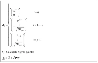
After revising the formulas of simplex sigma set UT, the new flow is shown in Figure 1.
15
1) Choose initial weight 0≤W0 ≤1
2) Choose weight sequence:
0
1 2
1
1
1 2
2
2 3, 1
n
i i
W i
W W i
W i n
− −
=
= =
= +
3) Initial vector sequence:
[ ]
10 0
σ = , 1
1
1
1 2W
σ = −
, 1 2
1
1 2W
σ =
1 0
1
1
1
1
0 0
1 1,
2
0
1 1
2
j
j i j
i
j
j
j
i
i j
W
i j
W
σ
σ σ
−
−
+ −
+
=
= − =
= +
5) Calculate Sigma points:
n i = +X σi
χ P
Fig. 1 The revised simplex unscented transformation flow
1
The revised simplex unscented transformation satisfies the sum of weighs is unit one, and the
2
UT captures the mean and the covariance of the state after UT. For example, let X =
[
1;2;3;4;5;6]
,3
covariance matrix
6 6
1 0
0 1
P
×
=
which is 6 6× unit matrix,W0=0.5,we can calculate the
4
mean and covariance after UT, which are:
5
[
1;2;3;4;5;6]
X χμ = = ,
6 6
1 0
0 1
P χχ
×
= =
.
6
However, this kind of UT method has the problem that the radius which bounds the sphere of
7
the sigma points is2n/2. Therefore, at even relatively low dimensions there are potential problems 8
with numerical stability.
9
3.2. Spherical Simplex Unscented Transformation
10
The spherical simplex unscented transformation was developed with the goal of rearranging the
11
sigma points of the simplex algorithm in order to obtain better numerical stability [12]. The sigma
12
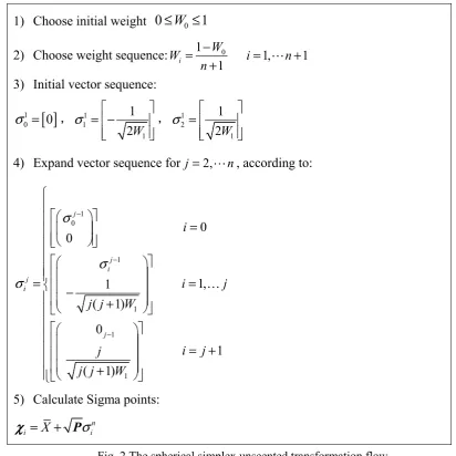
points are lie in the hypersphere with radius of n/ (1−W0) . The algorithm flow of spherical
13
unscented transformation is shown in Figure 2.
1) Choose initial weight 0≤W0≤1
2) Choose weight sequence: 1 0 1, 1
1
i
W
W i n
n
−
= = +
+
3) Initial vector sequence:
[ ]
10 0
σ = , 1
1
1
1 2W
σ = −
, 1 2
1
1 2W
σ =
4) Expand vector sequence for j=2,n, according to:
1 0
1
1
1
1
0 0
1, 1
( 1)
0
1 ( 1)
j
j i j
i
j
i
i j
j j W
i j
j
j j W
σ
σ σ
−
−
−
=
= = −
+
= + +
5) Calculate Sigma points:
n i = +X σi
χ P
Fig. 2 The spherical simplex unscented transformation flow
1
According to the statements of Menegaz [15], the spherical simplex UT cannot capture the
2
mean and covariance of the state after UT. Actually, the formulas in Table I of [15] were not
3
consistent with Julier’s [12], the readers can simply find it by making a comparison between the
4
formulas in Fig. 2 here with Table I in the corresponding paper of [15]. Take the same example of
5
his paper, let the mean value before UT be X =
[ ]
0 2 1× ,covariance be 1 0 0 1P=
,W0=0.5, then
6
we can calculate the mean and covariance after UT are, 0
[ ]
0 2 1 0χ
μ = = ×
and
1 0 0 1
χχ
=
,7
respectively.
8
Actually, the mean and the covariance are all capture the mean and the covariance of the state
9
after UT.
10
From the above statements, we can say that the conclusion only the minimum set proposed by
11
Menegaz [16] matching the mean and the covariance matrices (CM) of the system state is not very
accurate.
1
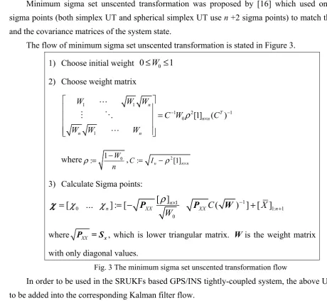
3.3. Minimum Sigma Set Unscented Transformation
2
Minimum sigma set unscented transformation was proposed by [16] which used only n +1
3
sigma points (both simplex UT and spherical simplex UT use n +2 sigma points) to match the mean
4
and the covariance matrices of the system state.
5
The flow of minimum sigma set unscented transformation is stated in Figure 3.
6
1) Choose initial weight 0≤W0≤1
2) Choose weight matrix
1 1
1 2 1
0
1
[1] ( )
n
T n n
n n
W W W
C W C
W W W
ρ
− −
×
=
where : 1 W0
n
ρ = − , : 2[1]
n n n
C = I −ρ ×
3) Calculate Sigma points:
1 1
0 1: 1
0 [ ]
[ ... ] : [ n ( ) ] [ ]
n XX XXC X n
W
ρ
χ
χ
× −+
= = − +
χ
P P Wwhere P = SXX x, which is lower triangular matrix. Wis the weight matrix
with only diagonal values.
Fig. 3 The minimum sigma set unscented transformation flow
7
In order to be used in the SRUKFs based GPS/INS tightly-coupled system, the above UTs have
8
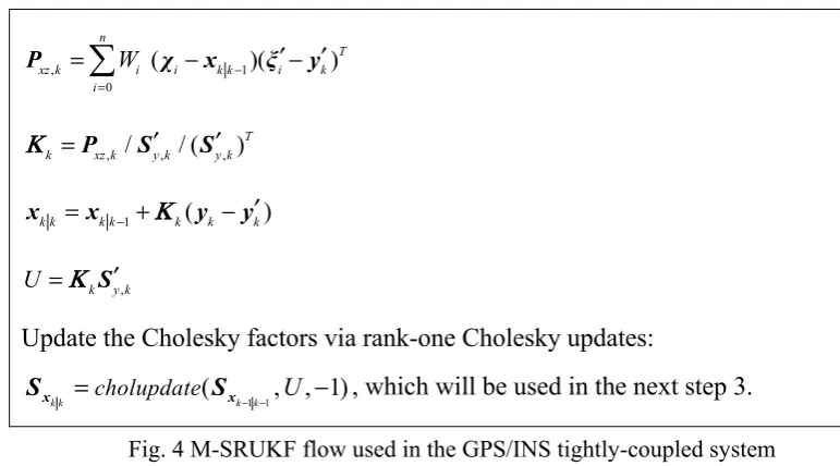
to be added into the corresponding Kalman filter flow.
9
Here we only give the Kalman filter flow of the M-SRUKF used in the GPS/INS
10
tightly-coupled system, which is shown in Fig. 4. Actually, the difference among the filters (SRUKF,
11
S-SRUKF, SS-SRUKF, M-SRUKF) are just lie in the UT procedure.
12
1) Initial values of state and the state covariance of the 17 states in (7):
{
}
0 0
0 0 0
0 0 [( 0 0 ˆ )( 0 0 ˆ ) ]
T
chol E
= , x = − −
x x S x x x x
2) Initial coefficients for M-SRUKF:
Choose0≤W0 ≤1.
Set : 1 W0
n
ρ = − , : 2[1]
n n n
1
( ,..., n).
W =diag W W
For 1 2 1
0 ,
1,..., : [ [1] ( T) ]
i n n i i
i n W C W− ρ C −
×
= =
which is the weight that associates with i-th sigma point 3) Time update equations:
Propagate directly through state transition function:
1 1 1
1 1
1 1 1
1/2
( )
k k k k
k k k k
k k k k k
k
qr
− − −
− −
− = − − =
=
x x
x x
x F x
S F S
S S Q
k
F is the systematic matrix after discretization.
The state of the filter is the form of error, so the mean and covariance can be predicted directly without using the spreading sigma points. This may save the computation time greatly.
1 1 1
k k− = k k− −k
x x
S F S is derived from
1 1 1
k k− = k k− −k k′
x x
P F P F , where
1 1
k− −k
x
P is the covariance matrix of the state. qr
( )
⋅represents QR decomposition function. 4) Calculate Sigma points:
1 1 1 1
1 1
0 1 1 1: 1
0 [ ]
[ ... ] : [ ( ) ] [ ]
k k k k
n
n C W k k n
W
α
χ
χ
− − × − − −+ − −
= = −Sx Sx + x
χ
,The column vectors of χ are the sigma point vectors, kis the iteration
time starts from 1.
5) Measurement update equations:
Propagate through observation function (13):
( )
h
′ =
ξ
χ
Calculate Mean of the predicted measurements:
0
n
k i
i i
W
= ′ =
′y ξ
Calculate the covariance value of the measurements:
1/ 2 , ( ( 1:2 ) )
y k qr Wi n k
′ = ′ − ′
S ξ y R
, ( , , 0 , 0 )
y k cholupdate y k k W
′ = ′ ′− ′
S S ξ y
, 1 0
( )( )
n
T
xz k i i k k i k
i
W −
=
′ ′
=
− −P χ x ξ y
, / , / ( , )
T k =Pxz k Sy k′ Sy k′
Κ
1 k( k k) k k = k k− + − ′
x x Κ y y
,
k y k
U =Κ S′
Update the Cholesky factors via rank-one Cholesky updates:
1 1
( , , 1)
k k =cholupdate k− −k U −
x x
S S , which will be used in the next step 3.
Fig. 4 M-SRUKF flow used in the GPS/INS tightly-coupled system
1
4. Pseudo Satellite Measurements
2
GNSS signals are vulnerable to disruption by environmental and man-made interference, so
3
they would not meet all of the emerging performance requirements of navigation. The navigation
4
error may be large even for the GPS/INS coupled system when there is no enough observation
5
information. One simple way to solve this problem is to add more constraints for the observation
6
equations. A pseudo-GPS mechanism was proposed by [30] for the loosely-coupled GPS/INS system.
7
The pseudo-GPS method can afford artificial pseudoranges and pseudorange rates for calculating the
8
GPS receiver position and velocity. The extra pseudo measurements can be added to enhance the
9
position and velocity solution when there is no enough observed satellites.
10
The pseudo-GPS satellites can be taken together with the true satellites, viewed by the receiver.
11
For example, the radio navigation station can work as a pseudo satellite. The signal sent by radio
12
navigation station will be received by the moving receiver, and then the pseudoranges and
13
pseudorange rates are created.
14
Assumed i-th pseudo-satellite is fixed at rpseu i( ) =(xpseu,ypseu,zpseu)( )i in ECEF frame, then the
15
pseudorange updated by model can be written as:
16
( ) ( ) sins ( ) sins r
ˆ [ (ˆ c)] [T (ˆ c)]
r i pseu i pseu i u p a
P = r − r −δr r − r −δr +c tδ +w (14)
17
The pseudorange rate updated by model can be written as:
18
( ) sins
( ) ( ) sins r
( ) sins ( ) sins
ˆ
[ ( )]
ˆ [ (ˆ )]
ˆ ˆ
[ ( )] [ ( )]
c T
pseu i c
r i c T c pseu i ru v a
pseu i pseu i
V δ δ c tδ w
δ δ
− −
= − − + +
− − − −
r r r
v v v
r r r r r r (15)
19
Furtherly, in order to be used in the SRUKFs, the observation equations set by pseudo-satellite is
20
described as:
{
}
( ) ( ) ( ) sins ( ) sins r
( ) sins
( ) sins ( ) sins
( ) ( )
ˆ [ (ˆ (7 : 9))] [ (ˆ (7 : 9))] (16)
ˆ
[ ( (7 : 9))]
ˆ [ (ˆ (7 : 9))] [ (ˆ
ECEF T ECEF
r i r i pseu i Lh pseu i Lh p a
ECEF T
pseu i Lh
ECEF T
pseu i Lh pseu i Lh
r i r i
P P C C w
C
C C
V V
λ λ
λ
λ λ
−
Δ = − − − − + +
− −
− − − −
Δ = −
r r X r r X X
r r X
r r X r r r
( ) sins
(7 : 9))]
ˆ
[ ( (4 : 6))] (17)
ECEF
v a ECEF
pseu i NED
w
C
⋅
+
− − +
X
v v X X
(16)
1
In (16), ( )
( ) ( )( ) ( ) 1,...
r
r i r i ori i n
P =P +δP +δt − +T ε , ( )
( ) ( )( ) ( ) 1,...
r
r i r i ori i n
V =V +δP +δf − +T ζ , where
2
( )( )
r i ori
P is the original pseudorange directly from the observation file of the rover which is the
3
distance between the rover and the pseudo satellite; δP( )i and δP( )i , known as the Sagnac or
4
Earth-rotation correction of pseudorange and pseudorange rate, usually can be ignored since the
5
rover is not far away from the pseudo satellite station;
δ
t( )r is the clock error of the pseudo satellite;6
T is troposphere propagation errors, which usually can be ignored, since when the rover is not far
7
away from the pseudo satellite station, it’s error is quite small ; δ f( )r is pseudo satellite clock drift;
8
Tis troposphere error range rate of T , which is also very small in general, so they can be ignored;
9
r
p a
w is the measurement noise of pseudorange; wv ar is the measurement noise of pseudorange rate;
10
1,...n
ε and ζ1,...n are errors that are not explicitly modeled or measured.
11
5. Experiments of UAV
12
Simulations below are based on the post-processing of the UAV field test data. In the UAV
13
experiment, the reference result was obtained from difference GPS and INS coupled system.
14
The initial conditions of the GPS/INS tightly-coupled system here are set as below.
15
The frequency of INS is 200Hz. The pure INS calculation is based on double-sample algorithm,
16
in which coning and sculling errors are compensated.
17
GPS updating frequency is 2Hz.
18
Observation length:1500s.
19
The initial parameters of SRUKFα equals 1, κequals -14, β equals 2 [14].
20
The initial weightsw0of M-SRUKF, S-SRUKF and SS-SRUKF are set as 0.5.
21
The initial error state covariance matrixP0is set as:
22
2 2 2 2 2 2
2 2 2 2 2 2
0
2 2 2 2 2
(0.5 ) (0.5 ) (0.5 ) (0.1 / ) (0.1 / ) (0.1 / ) (10 ) (10 ) (10 ) (10 / ) (10 / ) (10 / ) ;
(300 ) (300 ) (300 ) (25 ) (0.1 / )
m s m s m s
diag m m m h h h
g g g m m s
μ μ μ
;
=
P
The spectral density of measurement noise matrix is,
1
2
2 2
2
(2 / / ) 0 0 0
0 (0.5 / / ) 0 0
0 0 (1 / / ) 0
m m
m m
n n
m s Hz
m s Hz
m s Hz
×
×
× =
I
I R
I
2 2
0 0 0 (0.5 /m s / Hz) n n×
I
2
The spectral density of process noise matrix is,
3
2 2 2
2 2 2
2 2 2
(0.1667 / ) (0.1667 / ) (0.1667 / )
(300 / ) (300 / ) (300 / )
(25 / / ) (0.1 / / )
h h h
diag g Hz g Hz g Hz
m s Hz m s Hz
μ μ μ
=
q
4
The discretization form of q is Q, which obeys Q = TGqGT, where Tis the discretization
5
time and G is the shaping matrix of noise.
6
The flight trajectory of the UAV is as Fig. 5 describes.
7
8
Fig. 5. Trajectory of the UAV
9
5.1.Comparisons among EKF , SR-UKFs
10
Comparisons are made among EKF, standard SRUKF and reduced sigma point SRUKFs
11
GPS/INS tightly-coupled systems in two scenarios. In the first scenario, seven satellites are visible
12
during the whole flight of UAV. The mean and the standard deviation of the absolute position errors
13
and the absolute attitude errors are shown in Table 1 and Table 2, respectively. Figure 6 show the
14
estimated biases of gyros and accelerometers. The second scenario is that from 800s to 1000s there
15
are only three visible satellites available; the mean and the standard deviation of the absolute position
16
errors and the absolute attitude errors are shown in Table 3 and Table 4, respectively.
17
18
19
20
z(
Table 1 Mean values and standard deviation values of the absolute position errors when there are seven visible satellites
1
during the whole time (m)
2
Algorithms Latitude Longitude Height
Mean Std. Dev. Mean Std. Dev. Mean Std. Dev.
EKF 0.21 1.32 0.62 0.85 1.67 1.92
SRUKF 0.11 1.24 0.18 0.64 0.95 1.23
S-SRUKF 0.11 1.24 0.18 0.65 0.95 1.23
SS-SRUKF 0.11 1.24 0.18 0.65 0.95 1.23
M-SRUKF 0.11 1.24 0.18 0.65 0.95 1.23
3
Table 2 Mean values and standard deviation values of the absolute attitude errors when there are seven visible
4
satellites during the whole time (deg)
5
Algorithms Roll Pitch Yaw
Mean Std. Dev. Mean Std. Dev. Mean Std. Dev.
EKF 0.01 0.06 0.04 0.05 0.33 0.17
SRUKF 0.01 0.05 0.04 0.04 0.33 0.18
S-SRUKF 0.01 0.06 0.04 0.05 0.33 0.19
SS-SRUKF 0.01 0.06 0.04 0.05 0.33 0.18
M-SRUKF 0.01 0.06 0.04 0.05 0.33 0.18
6
Table 3 Mean values and standard deviation values of the absolute position errors when there are only three visible
7
satellites during 800s to 1000s (m)
8
Algorithms Latitude Longitude Height
Mean Std. Dev. Mean Std. Dev. Mean Std. Dev.
EKF 5.54 20.07 2.18 9.72 7.37 20.07
SRUKF 4.19 14.44 1.92 6.71 2.98 12.79
S-SRUKF 4.19 14.42 1.92 6.70 2.97 12.78
SS-SRUKF 4.19 14.42 1.92 6.70 2.97 12.78
M-SRUKF 4.19 14.42 1.92 6.70 2.97 12.78
9
Table 4 Mean values and standard deviation values of the absolute attitude errors when there are only three visible
10
satellites during 800s to 1000s (deg)
11
Algorithms Roll Pitch Yaw
Mean Std. Dev. Mean Std. Dev. Mean Std. Dev.
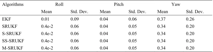
EKF 0.01 0.09 0.04 0.06 0.37 0.26
SRUKF 0.4e-2 0.06 0.04 0.05 0.34 0.20
S-SRUKF 0.4e-2 0.06 0.04 0.05 0.34 0.20
SS-SRUKF 0.4e-2 0.06 0.04 0.05 0.34 0.20
M-SRUKF 0.4e-2 0.06 0.04 0.05 0.34 0.20
Fig. 6 (a). The estimated gyro constant biases Fig. 6 (b). The estimated accelerometer constant biases
1
It can be seen from Table 1, in terms of the absolute position errors, all the SRUKFs (including
2
the reduced sigma point SRUKFs) have only slightly higher accuracy than EKF in the first scenario
3
when GPS observation information is enough. Also, the SRUKFs and EKF show the similar
4
accuracy in terms of the attitude estimation which is shown in Table 2.
5
In the second scenario, however, when GPS signal is deficient, the SRUKFs performed distinct
6
higher accuracy than EKF in terms of the mean and the standard deviation of both the absolute
7
position and attitude errors, which can be seen from Table 3 and Table 4.
8
All the results from Table 1 to Table 4 show that the filters SRUKF, S-SRUKF, SS-SRUKF and
9
M-SRUKF have nearly the same accuracy in the GPS/INS tightly coupled system, because they use
10
nearly the same mechanization except that the number of sigma points is different. M-SRUKF uses
11
only n+1sigma points, while both S-SRUKF and SS-SRUKF use n+2 sigma points, the standard
12
SRUKF uses 2n+1 sigma points. From this point, M-SRUKF is the best filter here, since it has only
13
nearly half computational cost of the standard SRUKF but still has higher accuracy than EKF.
14
The estimation of gyro and accelerometer constant biases of EKF and SRUKFs in Fig. 6 show
15
that, all of them can estimate the constant biases successfully. But all the SRUKFs have faster
16
convergence rate than EKF, which is to say that the latter has longer estimation time, which can be
17
seen explicitly from the y direction gyro, x, y and z direction accelerometers.
18
Meanwhile, comparisons between Fig. 7 (a) and Fig. 7 (b) (the second scenario) show that,
19
M-SRUKF has faster convergence rate than EKF when the number of visible satellites recovered
20
from partial outages to normal level.
21
22
23
24
0 500 1000 1500
-20 -10 0 10
x
(deg/hr)
Gyro constant bias
0 500 1000 1500
-10 -5 0 5
y
(deg/hr)
0 500 1000 1500
time (s) -20
-10 0 10
z
(deg/hr)
EKF SRUKF SS-SRUKF S-SRUKF M-SRUKF
200 400 -4
-2 0 500 1000 1500
-0.02 0
0.02 Accelerometer constant bias
0 500 1000 1500
-0.02 0 0.02
0 500 1000 1500
time (s)
-0.01 0 0.01
Fig. 7 (a). EKF GPS/INS tightly-coupled position errors (there are GPS lost from 800 to 1000s)
Fig. 7 (b). M-SRUKF GPS/INS tightly-coupled position errors (there are GPS lost from 800 to 1000s)
1
Figure 7 indicates that the M-SRUKF (here only shows M-SRUKF based GPS/INS
2
tightly-coupled errors, since other SRUKFs have similar accuracy with M-SRUKF) has faster
3
convergence rates than EKF when the number of visible satellites is recovered from three to seven.
4
EKF takes more than 100s longer than M-SRUKF to recover to normal navigation and location
5
(positon errors less than 10m), which means that the M-SRUKF is more effective than EKF. Similar
6
comparisons can also be seen in a spacecraft relative navigation example [28], which also showed
7
that SRUKF has faster convergence rate than EKF.
8
Simulations above indicates that M-SRUKF is a better mean for the GPS/INS tightly-coupled
9
system, considering both from the accuracy and computation cost.
10
5.2. Pseudo-satellite Aided M-SRUKF
11
Figure 7 (b) displays that there is still maximum error 85m for the M-SRUKFtightly-coupled
12
system position error, which is a large error of normal navigation. In this section, a pseudo-satellite is
13
introduced to improve the navigation accuracy of M-SRUKF GPS/INS tightly-coupled system when
14
there are only three visible satellites from 800s-1000s.
15
Assume the pseudo satellite (xpseu,ypseu,zpseu) is fixed at ECEF frame, which is about 30km
16
away from the rover in y direction. In order to avoid the mutual signal interference, the minimum
17
range between each pseudo satellite is 54km [31]. The problem of designing the whole pseudo
18
satellite network is not in the scope of this paper; readers can reference the paper [24].
19
The observation equations driven by pseudo-satellites are as (16) describes. δP( )i and δP( )i are
20
ignored since the rover is not far away from the pseudo satellite stations; Assume the clocks between
21
the rover and the pseudo satellites are synchronized; Troposphere propagation errors, which are quite
small, are ignored, since the rover is not far away from the pseudo satellite station; wp ar and wv ar
1
are initialized at the beginning of this chapter.
2
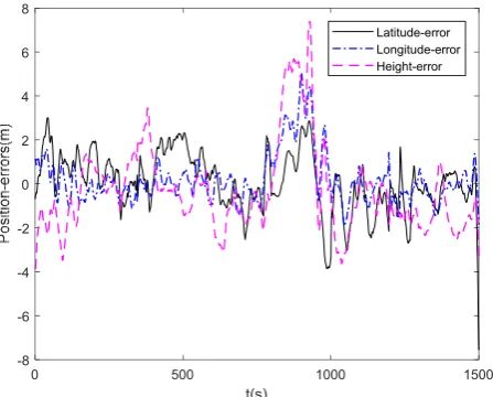
Positioning results are shown in Figure 8. It shows that the M-SRUKF GPS/INS tightly-coupled
3
system goes back to normal navigation level (with only maximum height error 7.2m) with the aiding
4
of pseudo-satellites.
5
6
Fig. 8. M-SRUKF GPS/INS tightly-coupled position errors (one pseudo-satellite aided)
7
In theory, more accurate results can be obtained with more pseudo-satellites, especially when
8
there is no enough observation information. As well as that, the geometry between pseudo-satellites
9
and the rover also affects the navigation results, which is beyond the scope of this paper.
10
11
6. Conclusions
12
In this paper, some questionable formulas and conceptual comments of previous UT methods,
13
which use less than 2n sigma points, are revised. Real UAV data was used for the performance
14
comparison among EKF, SRUKF and S-SRUKF, SS-SRUKF and M-SRUKF based GPS/INS
15
tightly-coupled systems. Results showed that all the SRUKFs had only slightly higher accuracy than
16
EKF when GPS observation was enough. However, SRUKFs showed distinct higher position
17
accuracy than EKF when GPS signal was deficient. All the SRUKFs had nearly the same accuracy
18
for the GPS/INS tightly-coupled system. But the reduced sigma point SRUKFs’ computation cost
19
were greatly saved, since they had only nearly half the computational cost of standard SRUKF. All
20
the SRUKFs have faster convergence rates than EKF when GPS signals were recovered from partial
21
outages to normal level. Meanwhile, SRUKFs have faster convergence rates in estimating the
22
constant biases of gyros and accelerators than EKF. To trade off between accuracy and computation
23
cost, M-SRUKF is a better mean than other filters for the GPS/INS tightly-coupled system.
24
Pseudo-satellite aided mechanism was introduced to improve the M-SRUKF GPS/INS
25
0 500 1000 1500
t(s)
-8 -6 -4 -2 0 2 4 6 8
tightly-coupled system when GPS outage occurs. Simulations showed that this aiding mechanism
1
worked well.
2
Acknowledgments
3
This work was supported by the National Natural Science Foundation of China (No.61573371
4
and No.61773394) and National University of Defense Technology Advanced Research Programs
5
(No.JC14-03-04). The authors also want to express their sincere thanks for the support of China
6
Scholarship Council (CSC, File No. 201603170338).
7
Conflicts of Interest
8
The authors declare no conflict of interest.
9
References
10
1.Petovello, Mark G. Real-time integration of a tactical-grade IMU and GPS for high-accuracy
11
positioning and navigation. 2003.
12
2.Wendel J, Maier A, Metzger J, et al. Comparison of extended and sigma-point Kalman filters for
13
tightly coupled GPS/INS integration. AIAA paper, 2005, 6055.
14
3.Wendel, J., Metzger, J., Moenikes, R., Maier, A., & Trommer, G. F. . A performance comparison of
15
tightly coupled GPS/INS navigation systems based on extended and sigma point Kalman
16
filters. Navigation, 2006, 53(1), 21-31.
17
4.El-Sheimy, N., E.-H. Shin, et al. Kalman filter face-off: Extended vs. unscented Kalman filters for
18
integrated GPS and MEMS inertial. Inside GNSS 2006, 1(2): 48-54.
19
5.Gross, J., Y. Gu, et al. A Comparison of Extended Kalman Filter, Sigma-Point Kalman Filter, and
20
Particle Filter in GPS/INS Sensor Fusion. AIAA Guidance, Navigation, and Control Conference,
21
American Institute of Aeronautics and Astronautics, 2010.
22
6.Li, Y., C. Rizos, et al. Sigma-Point Kalman Filtering for Tightly Coupled GPS/INS Integration.
23
Navigation 2008, 55(3): 167-177.
24
7.Yang C, Shi W, Chen W. Comparison of unscented and extended Kalman filters with application
25
in vehicle navigation. The Journal of Navigation, 2017, 70(2): 411-431.
26
8.Julier S J, Uhlmann J K. A new extension of the Kalman filter to nonlinear systems. Int. symp.
27
aerospace/defense sensing, simul. and controls. 1997, 3(26): 182-193.
28
9.Wu, Y., Hu, D., Wu, M., & Hu, X. A numerical-integration perspective on Gaussian filters. IEEE
29
Transactions on Signal Processing, 2006, 54(8), 2910-2921.
30
10. Li, Y., C. Rizos, et al. Sigma-Point Kalman Filtering for Tightly Coupled GPS/INS Integration.
31
Navigation 2008, 55(3): 167-177.
32
11. Julier, S. J., & Uhlmann, J. K. Reduced sigma point filters for the propagation of means and
33
covariances through nonlinear transformations. In Proceedings of the 2002 American Control
34
Conference (IEEE Cat. No. CH37301) 2002, May, (Vol. 2, pp. 887-892). IEEE.
35
12. Julier, S. J. The spherical simplex unscented transformation. In American Control Conference,
36
2003. Proceedings of the 2003 (Vol. 3, pp. 2430-2434). IEEE.
37
13. Wan-Chun, L., Ping, W., & Xian-Ci, X. A novel simplex unscented transform and filter. In
Communications and Information Technologies, 2007. ISCIT'07. International Symposium on (pp.
1
926-931). IEEE.
2
14. Merwe, R. V. d. and E. A. Wan. The square-root unscented Kalman filter for state and
3
parameter-estimation. 2001 IEEE International Conference on Acoustics, Speech, and Signal
4
Processing, (ICASSP '01).
5
15. Menegaz, H. M., Ishihara, J. Y., Borges, G. A., & Vargas, A. N. A systematization of the
6
unscented Kalman filter theory. IEEE Transactions on Automatic Control, 2015, 60(10),
7
2583-2598.
8
16. Menegaz, H. M., Ishihara, J. Y., & Borges, G. A. A new smallest sigma set for the Unscented
9
Transform and its applications on SLAM. In 2011 50th IEEE Conference on Decision and Control
10
and European Control Conference (pp. 3172-3177). IEEE.
11
17. Penn, T. R. All Source Sensor Integration Using an Extended Kalman Filter (No.
12
AFIT/GE/ENG/12-32). AIR FORCE INST OF TECH WRIGHT-PATTERSON AFB OH
13
GRADUATE SCHOOL OF ENGINEERING AND MANAGEMENT, 2012.
14
18. Chiang, K. W. INS/GPS Integration Using Neural Networks for Land Vehicular Navigation
15
Applications, Department of Geomatics Engineering, The University of Calgary, Calgary, Canada,
16
UCGE Report 20209, 2004.
17
19. Chiang, K. W., & Huang, Y. W. An intelligent navigator for seamless INS/GPS integrated land
18
vehicle navigation applications. Applied Soft Computing, 2008, 8(1), 722-733.
19
20. Semeniuk, L., & Noureldin, A. Bridging GPS outages using neural network estimates of INS
20
position and velocity errors. Measurement science and technology, 2006, 17(10), 2783.
21
21. Li, Z., Wang, J., Li, B., Gao, J., & Tan, X. GPS/INS/Odometer integrated system using fuzzy
22
neural network for land vehicle navigation applications. The Journal of Navigation, 2014, 67(06),
23
967-983.
24
22. Jiang, W., Li, Y., Rizos, C., & Barnes, J. Flight evaluation of a locata-augmented multisensor
25
navigation system. Journal of Applied Geodesy, 2013, 7(4), 281-290.
26
23. Jiang, W., Li, Y., & Rizos, C. On-the-fly Locata/inertial navigation system integration for precise
27
maritime application. Measurement Science and Technology, 2013, 24(10), 105104.
28
24. Yang, L., Li, Y., Jiang, W., & Rizos, C. Locata Network Design and Reliability Analysis for
29
Harbour Positioning. Journal of Navigation, 2015, 68(02), 238-252.
30
25. Bar-Itzhack, I. Y., & Berman, N. Control theoretic approach to inertial navigation systems.
31
Journal of Guidance, Control, and Dynamics, 1988, 11(3), 237-245.
32
26. Jiang, J., Yu, F., Lan, H., & Dong, Q. Instantaneous Observability of Tightly Coupled SINS/GPS
33
during Maneuvers. Sensors, 2016, 16(6), 765.
34
27. Liu, Z., Chen, J., Yao, X., Song, C., & Wang, Y. An improved square root unscented Kalman
35
filter for projectile's attitude determination. In 2010 5th IEEE Conference on Industrial Electronics
36
and Applications (pp. 1747-1751). IEEE.
37
28. Tang, X., Yan, J., & Zhong, D. Square-root sigma-point Kalman filtering for spacecraft relative
38
navigation. Acta Astronautica, 2010, 66(5), 704-713.
39
29. Simon, D. Optimal state estimation: Kalman, H infinity, and nonlinear approaches. John Wiley
40
& Sons. 2006
41
30. Klein, I., S. Filin, et al. Pseudo-GPS in INS/GPS Loosely-Coupled Integration Approach.
42
31. Wang Guangyun, Guo Bingyi, Li Hongtao. Positioning technology of DGPs and its application.
43
Beijing: Publishing House of Electronics Industry, 1996.