Application Of Shallow Seismic Refraction To Detect Engineering Problems, Madinaty City, Egypt.

146

Application of Shallow Seismic Refraction To Detect

Engineering Problems, Madinaty City, Egypt.

Abdel Hafeez Th. H.* ,Thabet H. S.*, Diaa Hamed*,Azab M.A.* Basheer.A.A.** And Abdel Qawi S.R.***.

*Geology Department, Faculty of Science, Al-Azhar University, Cairo, Egypt. ** Geology Department, Faculty of Science, Helwan University, Cairo, Egypt.

***Aloqbi Cosultant Engineering Office,Jeddah.KSA.

31TU

[email protected]U31T

31TU

[email protected]U31T

ABSTRACT

Applied geophysical techniques in engineering investigation are of growing interest in

Egypt now, especially after the October 1992 earthquake and property damage in Manshiet

Naser August 2008 and its destructive impact on some buildings in new cities. Finding the exact

depth to the bedrock and its lithological type, the depth to the groundwater, the lateral changes in

lithology, and detecting faults, fissures, or demerits are the main objectives to achieve

engineering sites. Shallow seismic refraction surveys taken at two selected sites in the study area,

to determine their characteristics before carrying out any constructions. Twenty-four seismic

refraction profiles taken along the study area in preliminary procedure. Subsurface geological

features that make construction problems identified, such as geologic structures and clay layers.

Engineering properties of subsurface strata studied. Three geoseismic layers, ranging between

(827 and 848.7 m/s), (829 and 848.7 m/s) and (860 and 1553.7 m/s), have been indicated using

seismic primary wave velocity distribution. The shear wave velocity distribution in three

geoseismic layers are ranging between (436.1 and 446.9 m/s), (437.1 and 446 m/s) and (452.6

and 6-799.4 m/s). The obtained results indicate that the surface layer indicate weathered

limestone with sand and gravel, and the first layer composed of limestone, while the second

layer is represented by the dolomitic limestone. The estimated thicknesses of three layers vary

laterally, ranging from 0.50 m to 1 m for the surface layer, from 9 m to 14 m for the first layer,

and up to 14 m for the second layer. Different parameters such as shear wave velocity, rock

147 index and stress ratio have been calculated using a fundamental equation. The description of

materials that found within the study area are competent materials and rated as moderate to good

competent materials.

Keywords: Seismic refraction profiles, Primary wave velocity, Shear wave velocity and Poisson’s ratio.

INTRODUCTION

Today, shallow geophysical techniques are considered as one of the most accurate

and cost effective methods used in engineering, environmental investigations and archaeological

studies. This achievments because of the expanding the interpretive skills of the geophysists and

increasing the capabilities of the engineer and geologists through the use of basic geophysical

principles. Seismic refraction technique, in especial, has faced during the 30 years an increased

application in the study of engineering site selected. This includes major projects such as

delineating solution cavities in foundation rocks, construction of hydroelectric power plants,

subways, road, and tunnels. A seismic method has been coming out as a commanding

implements in computing the elastic moduli from which their elastic deformation can be

estimated for civil engineering projects (Stumpel et.al 1984; Harden and Drnevich 1972; David

and Taylor Smith 1979).

The interpretation of dynamic elastic moduli determined from the velocity measurements

of the foundation rock shown in the natural (earthquake) and the artificial (machine) cyclic

dynamic loading creates additional load, which is added to the building load which exceeds the

ultimate bearing capacity of the rock materials (Bowles 1984). Soil competence scales are not

enough for site machine foundation assessment in both quiet and earthquake active areas. From

the view engineering point, soil is defined as “the material overlying the bedrock produced by

rock weathering”. Soil is the unconsolidated material of the earth’s crust used to build upon or

used as a construction material. The soil mechanical properties depend on the elastic properties

of the rock materials, which may be evaluated from the conventional techniques or from the

geophysical measurements (Sjorgren et.al 1979; Dutta 1984; Abed Elrhman et.al 1991&1992).

The Madinaty City is using the shallow seismic refraction measurements (Compressional and

Shear wave's velocity). Madinaty City was intensively investigated by many scientists A.M.E.

148 considered a suitable tool to solve engineering site problems and delineate subsurface layering

and velocities.

The site response (transfer function) is evaluated through the Geotechnical parameters

(layer thicknesses, densities, P-wave velocities, shear wave velocities and damping factor of

layers), that are obtained from both the available Geotechnical boreholes and the seismic surveys

(Mohamed, 2003, 2009; and Mohamed et al., 2008). The P-wave velocity is obtained from the

seismic refraction survey and the S-wave velocity is deduced from the Multi-channel Analysis of

Surface Waves (MASW) survey. Prediction of ground shaking response at soil sites requires the

knowledge of stiffness of the soil, expressed in terms of shear wave velocity (Vs). This property

is useful for evaluating the site amplification (Borcherdt, 1994). The shear wave velocity of each

layer can be considered as a key element, so the determination of shear wave velocity is a

primary task of the current study of the considered area (Madinaty City), Figure (1).

149

GEOLOGIC SETTING

The surface geology in and around the studied area Figure (2) reveals

that, the older rocks are have been subdivided into two main rock units

by (Said,

1962). The oldest unit is made up of sands and gravels and was named by (Shukri,

1954) as the “Gebel Ahmar Formation” to refer to the Early Oligocene period. The

youngest rock unit is composed of basalt flows and referred to Late

Oligocene-Early Miocene period.

The younger rocks are the Upper Miocene beds at the southern side of Wadi

Hagul along the Gulf of Suez (Abdullah and Abdelhady, 1966). In the study area,

the Hagul Formation is made up of loose sand with small rounded flint pebbles and

fossil wood.

Gebel Ahmer Formation of Early Oligocene age followed unconformably by basaltic

intrusions of Late Oligocene age. Basaltic flows of Oligocene age followed unconformably by

150

Figure (2): Geological map of the New Cairo City and the study area (after EGSMA,1983)

METHODOLOGY AND DATA ACQUISITION

The seismic refraction survey was carried out through applying the forward, inline,

midpoint and reverse shootings to create the compressional waves (P-waves). The ground

refraction field work is executed in the interested area of the Twenty-four seismic refraction

profiles Figure (3).

151

Figure (3): Location map of seismic refraction spreads at the Madinaty City.

The P-waves are acquired by generating seismic energy using an energy source, sending

the created seismic waves inside the earth. The direct (head) and refracted (diving) waves are

detected through vertical geophones of 20 Hz and recorded using 24 channels signal

enhancement seismograph ‘‘Strata-View’’ as data logger. Most of the surveyed Twenty-four

seismic refraction profiles have a 100 meter long spread. The geophones, which were firmly

coupled to the ground, had 5 m fixed geophone spacing. The overall setup of compressional

waves is illustrated in Figure (4). The 24 channels signal enhancement seismograph

‘‘StrataView’’ of Geometrics Inc., USA, was employed for data acquisition along Twenty-four

152 layers down to at least 30 m, so the frequency content of the records had to be low enough to

obtain the phase velocities at longer wavelengths. The most important parts of the field

configurations are the geophone spacing and the offset range. The planar characteristics of

surface waves evolve only after a distance greater than the half of the maximum desired

wavelength (Stokoe et al., 1994).

Figure (4): Aseismograph model Strata View that used for data acquisition.

SEISMIC DATA PROCESSING AND RESULTS

The obtained results that the surface layer show withered sand and gravels, and show that

the velocity values of first layer indicate loose sand, while the second layer is represented by the

sands and gravels with some basalt flow, Figure (5a,b and c) show Time-Distance curve,

Geoseismic cross-section along profiles No. 2 as an example for all parts of the study area and

outcrop of the surface and first layers in the study area, where the results of the interpretation for

153

Figure (5a): Time-Distance curves along profile “2”.

Figure (5b) Geoseismic cross section No.“11” along profile “2”.

Figure (IV– 5c): Outcrop of the surface and first layers in the study area.

0.00 20.00 40.00 60.00 80.00 100.00 120.00

1 3 5 7 9 11 13 15 17 19 21 23 25

Normal Meddel. Reverse

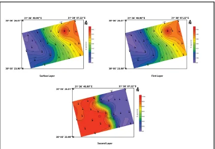
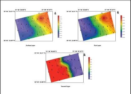
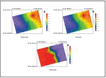
154 SEISMIC VELOCITIES

The velocities of the layers are determined by the reciprocal of the slope of each segment

of the time-distance curve. The P-wave and SH-wave velocities are determined in the four layers

for the 24 seismic sites of the studied area, Figures (6 and 7) show the P-wave and SH-wave

velocities distribution maps of the surface layers of the considered subsurface section. The

seismic primary wave velocity distribution indicated that there are three geoseismic layers

ranging between (827 and 848.7 m/s), (829 and 829-848.8 m/s) and (860 and 1553.7 m/s). The

shear wave velocity distribution are three geoseismic layeres ranging between (436.1 and 446.9

m/s), (437.1 and 446 m/s) and (452.6 and 799.4 m/s).

155

Figure (7): S-wave velocity distribution maps of the study area.

GEOTECHNICAL CHARACTERISITICS OF THE FOUNDATION MATERIAL

This study makes a view on the foundation rock in the study area using the shallow

seismic refraction measurements (Compressional and Shear wave's velocity).

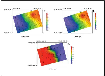
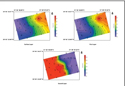
ELASTIC MODULI Poisson’s Ratio (σ):

The Poisson’s ratio of the three layers are shown in Figure (8). this ratio ranges between 0.3074 and 0.3081. Poisson’s ratio (σ) of the surface layer reveals that the lowest value is located in the western part and the northeastern part have higher values, also the first layer

reveals that lowest Poisson’s ratio (0.3074 ) is located in the western part, while the northeastern

part have a higher values (0.3082), the second layer reveals that lowest Poisson’s ratio (0.308) is

156

Figure (8): Poisson’s Ratio (σ) maps of the study area.

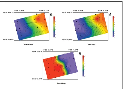
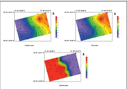
Kinetic Rigidity Modulus (μ):

Figure (9) shows the calculated rigidity modulus of the layers where the surface layer

(Withered sand and gravel) in the study area. The rigidity values of the surface layer range

between 376.6 dyn/cmP 2

P

and 416.2 dyn/cmP 2

P

. The minimum values are characterize the western,

these values increase gradually to the northeastern part of the area.

The rigidity values of the first layer range between 380.2 dyn/cmP 2

P

and 416 dyn/cmP 2

P

. The

minimum values are characterizing the western parts, these values increase gradually to the

northeastern part of the area too.

The rigidity modulus of the second layer in the study area. These values range between

437.8 dyn/cmP 2

P

and 4360 dyn/cmP 2

P

. The low values are observed in the eastern part where the less

competent and low rigidity materials. The low competent or more floppy materials are

experiential in the eastern parts of the study area. These values increase gradually to the western

157

Figure (9): Kinetic Rigidity Modulus (μ) maps of the study area.

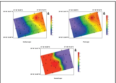
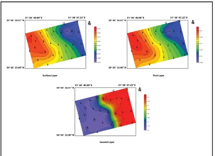
Kinetic Young’s Modulus (E):

Figure (10) illustrates the Young’s modulus distribution where the surface layer values

range between 984.9 dyn/cmP 2

P

and 1088.9 dyn/cmP 2

P

where the minimum values are observed in

the western sides of the study area. These values increase to the northeastern and eastern sides of

the study area. The Young’s modulus distribution of the first layer values ranges between 994.2

dyn/cmP 2

P

and 1089 dyn/cmP 2

P

. The low values are observed in the western parts of the study area;

these values increase gradually to the northeastern. The Young’s modulus distribution of the

second layer values ranges between 1145.9 dyn/cmP 2

P

and 11510 dyn/cmP 2

P

. The low values are

observed in the eastern part of the study area; these values increase gradually to western corner

158

Figure 10: Kinetic Young’s Modulus (E)maps of the study area.

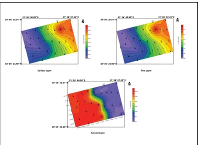
Kinetic Bulk Modulus (K):

The distribution of the Bulk modulus is shown in Figure (11). These values of the surface

layer range between about 852.3 dyn/cmP 2

P

and 945.8 dyn/cmP 2

P

. The minimums values of Bulk

modulus are observed in the western parts of the study area. While the maximum values are

observed in the northeastern corner of the study area. and the first layer; this modulus varies

from about 860.6 dyn/cmP 2

P

to 945.7 dyn/cmP 2

P

. The low values of this modulus are observed in

scattered sites as in the western parts, while the high values occupied in the northeastern part of

the area. The Young’s modulus distribution of the second values ranges between 997 dyn/cmP 2

P

and 10655 dyn/cmP 2

P

. The low values are observed in the eastern parts of the study area; these

159

Figure 11: Kinetic Bulk Modulus (K)maps of the study area.

STANDERD PENETRATION TEST (SPT) [N-VALUE]:

Figure (12) shows the distribution of the N-values .The surface layer values range between

102.6 and 110.3.The N-values of the first layer varies from 103.3 to 110.4; the minimum values

in western part of the study area reflect hard and dense competent soil. These values gradually

increase towards the northeastern parts. The distribution of the N-values of the second layer

values range between 114.4 dyn/cmP 2

P

and 606.9 dyn/cmP 2

P

. The low values are observed in the

160

Figure 12: N-valuesmaps of the study area.

MATERIAL COMPETENCE SCALES: The Material Index (ν):

The distribution of the material index of the surface layer in the study area is shown in

Figure (13), these values range from (-0.2296) to (-0.2324). These values of the material index in

the northeastern part, while these values increase towards the northeastern parts. The material

index in these parts indicate that the fairly to moderately Competent materials are located.

Figure (13) illustrates the distribution of the material index of the first layer in the study area. The material index values range between (-0.2299) to (-0.2325). the maximum values are located at the northwestern parts while the minimum values are located at the eastern and northeastern parts .

The distribution of the material index of the second layer in the study area is shown in

161 values are located at the northeastern and eastern parts while the minimum values are located at

the northwestern part of the study area.

Figure 13: The Material Index (ν)maps of the study area.

Concentration Index (Ci):

The distribution of the concentration index of the first layer is shown in Figure (14). This

index varies from 4.2455 to 4.2530 The low values are practicable in the eastern and

northeastern parts of the study area, these values indicate to relatively low competent to

moderately competent material. While the high values tend to appear in the western portion of

the study area, they indicate moderately competent to competent materials. Figure (14) shows

that the values of the concentration index in the first layer of the study area, these values show

range between 4.2448 and about 4.310245 the low values are observed especially in the eastern

and northeastern corners and increases gradually to the western part. These values indicate as

fairly to moderately competent materials. Figure (14) illustrates that the distribution of

162 between 4.12 and 4.1274 the maximum values are located at the eastern part while the minimum

values are located at the western part of the study area.

Figure 14: Concentration Index (Ci)maps of the study area.

Stress Ratio (Si):

Figure (15) shows the distribution of stress ratio of the surface layer. This value varies

between 0.4438 and 0.4453, the low values occupied the western parts, indicating as fairly to

moderate compact materials, while the high values are observed in the northeastern part of the

study area, reflecting relatively less-compact to fairly moderate materials. The division of the

stress ratio of the first layer along the study area is illustrated in Figure (15). The values of this

ratio show range between 0.44545 and 0.44665 the low values dominant are observed in the

western part of the study area. These values increase gradually to the northeastern. These low

163 Figure (15) illustrates that the distribution of stress ratio of the second layer in the study

area. The stress ratio values range between 0.446 and 0.4704 the maximum values are located at

the western part while the minimum values are located at the eastern part of the study area.

Figure 15: Stress Ratio (Si)maps of the study area.

Density Gradient (ρ):

The distribution of the density gradient in the surface layer has been shown in Figure (16)

this figure shows little varies in the density gradient values from 0.0019 to 0.0020 . The

relatively low values are observed in the western parts of the study area, which indicate the

relatively moderate competent material. While the high values are observed in the northeastern

part of the study area, they reflect the fairly moderate competent materials in this part of the

164 Figure (16) shows the density gradient distribution in the first layer of the study area.

This map shows variation of the value ranges between about 0.0019 and about 0.0020 the very

low values are observed in the western parts of the study area reflecting moderate competent

material; while the values that indicate the high competent materials are observed in the

northeastern part of the study area that reflecting fairly to moderate competent materials.

Figure (16) illustrates that the distribution of density gradient of the second layer in the

study area. The density gradient values range between 0.0021 and 0.0068 the maximum values

are located at the western part while the minimum values are located at the eastern part of the

study area.

Figure 16: Density Gradient (Di)maps of the study area.

FOUNDATION MATERIALS BEARING CAPACITY Ultimate Bearing Capacity (Qult):

Figure (17) shows the calculated ultimate bearing capacity of the surface layer where the

values are generally moderate and ranged between 3078.5 K.Pa. and 3309.1 K.Pa. The relatively

165 indicates to low ultimate bearing capacity material. The high values of this parameter are

occupied in the eastern and northeastern parts of the study area, which indicate the moderate

ultimate bearing capacity material.

The distribution of the ultimate bearing capacity in the frist layer is shown in Figure (17).

This parameter’s values ranged from 3099.2 K.Pa to 3309 K.Pa, Where the relatively moderately

values of this parameter are observed in the western part of the study area, which may reflect the

moderately ultimate bearing capacity materials. The highest values of this parameter noted in the

northeastern part of the study area reflect the high ultimate bearing capacity materials.

Figure (17) illustrates that the distribution of ultimate bearing capacity of the second

layer in the study area. The ultimate bearing capacity values range between 3432 and 18207 the

maximum values are located at the western part while the minimum values are located at the

eastern part of the study area.

Figure 17: Ultimate Bearing Capacity (Qult)maps of the study area.

Allowable Bearing Capacity (Qa):

The distribution of the allowable bearing capacity (Qa) of the surface layer is shown in

Figure (18) this parameter values show range between 1539.2 K.Pa. and 1654.5 K.Pa., where the

166 gradually to the northeastern part that reflect the highest allowable bearing capacity materials in

the study area.

Figure (18) shows the distribution of the allowable bearing capacity of the first layer on

the study area. This parameter gives range from 1549.6 K.Pa to 1655.1 K.Pa. The noted

relatively low values of this parameter are observed in the western sides of the study area that

reflects moderately allowable bearing material. These values increase gradually to the

northeastern.

Figure (18) illustrates that the distribution of allowable bearing capacity of the second

layer in the study area. The allowable bearing capacity values range between 1716 and 9103 the

maximum values are located at the western part while the minimum values are located at the

eastern parts of the study area.

Figure 18: Allowable Bearing Capacity (Qa)maps of the study area.

167

Table (1 ) summarizing all the estimated elastic moduli, material competence, and foundation materials bearing capacity.

SUMMARY AND CONCLUSION

. The results obtained from the shot records and their interpretation indicate that, the P-wave

velocities are determined as follows: 1) very highly

weathered

having P-wave velocity range of (Vp1=827 - 848.7 m/s), in which the thickness of this layer is

ranged from 1m to 2 m.) The first layer velocity range of (Vp2=829-848.8 m/s), corresponds to

Loose sand with small rounded flint pebbles and fossil wood and the thickness of this layer from

9 m to 14 m), the second layer is characterized by a high seismic velocity range of

(Vp3=860-1553.7 m/s), that layer corresponds to Sands and gravels with some basalt flows. The Shear wave

velocities are illustrated in the velocity distribution maps. The surface layer is a thin layer must

be removed it, where the foundation level depth should be below it as well as being a less

competence layer where the velocity of the surface layer varies from (436.1 and 446.9 m/s). Also

Sands and Gravels with some Basalt

flow Loose Sand

with small Pebbles Withered

sand and gravels

Types of Layers

Depth 22m - Depth30m Depth 9m –Depth 15m

Surface layer

Depth of Layer

860-1553.7 829-848.8 827-848.7 P-Waves 452.6-799.4 437.1- 446 436.1 -446.9 S-wave 0.308-0.31995 0.3074-0.3082 0.3074-0.3081 Poisson’s Ratio (σ)

G EO TE C H N IC A L CH ARA CT E RI S IT

ICS Density gradient (ρ) _{0.0019-0.0020 0.0019-0.0020 0.0021-0.0068}

437.8-4360 380.2-416

376.6-416.2 Kinetic Rigidity Modulus (μ)

1145.9-11510 994.2-1089

984.9-1088.9 Kinetic Young’s Modulus (E)

997-10655 860.6-945.7

852.3-945.8 Kinetic Bulk Modulus (K)

114.4-606.9 103.3-110.4 102.6-110.3 N-values -0.233- -0.27981 -0.2299- -0.2325 -0.2296- -0.2324 Material Index (ν)

4.12-4.1274 4.2448-4.310245

4.2455-4.2530 Concentration Index (Ci)

0.446-0.4704 0.44545-0.44665

0.4438-0.4453 Stress Ratio (Si)

3432-18207 3099.2-3309

3078.5-3309.1 Ultimate Bearing Capacity (Qult)

1716-9103 1549.6-1655.1

168 the velocity of the first layer is ranged from (437.1 and 446 m/s)), where this layer is less

competence materials, this layer must be removed before putting the foundations for the

buildings which increase about 450 dyne/cm P 2

P

which can be used in entertainment facilities such

as swimming pools and similar. The velocity of the second layer is ranged from (452.6 and 799.4

m/s) where this layer has been bearing capacity for buildings ranging between 750 dyne / cm P 2

P

to 1200 dyne / cm P 2

P

. Using the fundamental equations, the following parameters such as: shear

wave velocity, rock density and material indices, which are represented by N-value, Poisson’s

ratio, material index and stress ratio can be calculated. This study suggests a classification to

foundation rock material in the study area for engineering purposes based on all the calculated

moduli and parameters.

REFERENCES

Abdallah, A.M., Abdelhady, F.M., (1966): Geology of Sadat area, Gulf of Suez. Journal Geology United Arab Republic. Vol. 10 (l), pp. l-22.

Abd Elrahman, M., Setto, I. And Elwerr (1991): Seismic refraction interpretations at the distinctive district 6P

th

P

.of October City. EGS. Proc. of the 9P th

P

Ann. Meet.3, PP. 229-242.

Abd Elrahman, M., Setto, I. And Elwerr (1992): Inferring mechanical properties of the foundation materials at the 2P

nd

P

industrial zone, Sadat City, from Geophysical measurement,

EGS. Proc. Of the 10P th

P

. Ann.Meet. 10, PP.50-62.

Adel M.E. Mohamed, A.S.A. Abu El Ata, F. Abdel Azim and M.A. Taha (2013): Site-specific shear wave velocity investigation for geotechnical engineering applications using

seismic refraction and 2D multi-channel analysis of surface waves NRIAG Journal of

Astronomy and Geophysics (2013) 2, 88–101.

Borcherdt, R.D., (1994): Estimation of site-dependant response spectra for design (methodology and justification). Earthquake Spectra 10,617–653.

Bowles, J. E., (1984): Physical and geotechnical properties of soils: New York, McGraw-Hill Book Company, 2nd Edition, 578 p.

David and Taylor Smith (1979): Applications of VRpR & VRs Rin Lithology. Geophysics;

Cambridge University Press, New York,860.

169

Harden and Dranevich (1972): Elastic Moduli Estimation for Civil Engineering; Cambridge University Press. 12-29.

Mohamed, A.M.E., Deif, A., El-Hadidy, SSheriff, R.E. (1991)

: Encyclopedic dictionary

of

Mohamed, A.M.E., (2003): Estimating earthquake ground motions at the Northwestern part of the Gulf of Suez. Egypt. Ph.D. Thesis,Fac. Sc., Ain Shams Uni. pp. 93–138.

Mohamed, A.M.E.,( 2009): Estimating the near surface amplification factor to minimize earthquake damage: a case study at west Wadi Hagoul area, Gulf of Suez. Egypt. J.

Geophys. Prospect. 57, 1073–1089. http://dx.doi.org/10.1111/j.1365-2478.2009.00796.x.

Said, R. (1962):The geology of Egypt. Elsevier, Amsterdam Pub. Co., P. 377.

Shukri, N. M., (1953):The geology of the desert east of Cairo, Bull. Inst. Desert, Egypt, 3,

2: pp. 89-105.

Sjogren, B., Ofsthus, A. and Sandberg, J. (1979): Seismic classification of rock mass qualities. Geophysical Prospecting, 27: P. 409-422.

Stumpel, M; Kahler, S; Meissner, R., and Nikereit, B., (1984): The use of seismic shear waves and compressional waves for lithological problems of shallow sediments.