c
Owned by the authors, published by EDP Sciences, 2018
From a reversible code to the quantum one: R-matrix
S. Mironov1,2,a
1INR RAS, Moscow, 60-letiya Oktyabrya 7a 2ITEP, Moscow, Bolshaya Chereomyshkinskaya 25
Abstract. This research has been carried out in collaboration with D.Melnikov, A.Mironov, A.Morozov and An.Morozov. We study the relation between quantum pro-gramming and knot theory. The general idea is that knot theory provides a special basis for unitary matrices. We suggest to use R-matrices of knot theory as universal gates in quantum code. We also examine basic operations in reversible programming.
1 Introduction
The definition of a quantum algorithm [1–3] is the following: quantum algorithm is a unitary matrix. This definition usually puzzles at first. We got accustomed to a classical coding, where algorithm is a sequence of operations, or a block diagram. We expect quantum code to be a straight-forward generalization of classical one, but it is formulated quite differently. The formal answer is that we
can formulate classical programming in terms of matrices. These are matrices of operators that act on a set of 0 and 1. But it is unnatural. The main reason is that quantum code is reversible, hence it’s natural to formulate it in a matrix form. On the other hand, the classical code is irreversible and we do not favor degenerate matrices. In other words, unlike classical, quantum programming has a group structure.
The less formal answer introduces classical reversible programming. It is a simple generalization of the standard classical programming. We add several additional bits to distinguish the same results of computation to make the code reversible. The classical reversible programming operates with the group of permutations (it acts on the initial set of states, all possible combinations of bits) i.e. non-degenerate matrices with one 1 in each column and each row. We describe a couple of examples in Sec 2.
The generalization to quantum programming is natural now: permutation group changes to unitary group. In other words, we allow a continuous change of a phase of a bit, and set of states becomes a vector space. Operationally one usually keeps operation of addition (CNOT) on two bits but changes operators on one bit, instead of Id=
1 0 0 1
and NOT=
0 1 1 0
one gets π
8 =
1 0
0 eiπ/4
and
Hadamard=
1 1 1 −1
gates.
On the other hand, it is not the only way to generalize the permutation group to unitary one. This way is preferred if we are going to use quantum computations for similar, addition-based problems.
But it is not always the case. One of the natural problems for quantum computer is the computation of knot invariants [4, 5]. Therefore, it is natural to generalize the permutation group via braid group and solutions of the Yang-Baxter equation [6]. An interesting possibility is to use group theoryR -matrices [7]. They become unitary at unimodular q when acting on the irreducible representations and this basis essentially simplifies the computations of the knot invariants [8], for example HOMFLY-PT polynomials (as a price, of course, it complicates some other codes). Sec 3 is devoted to the basics of R-matrices and its possible applications to quantum computing.
2 Reversible programming: examples
Let us start with the simplest operation, binary addition. Basically it is an addition of two numbers modulo 2, but it can be easily generalized to an addition of k-bit number and n-bit number modulo 2n (or 2k):
bit 1 bit 2 output
0 0 0
0 1 1
1 0 1
1 1 0
(1)
the matrix of the operator looks like:
1 0 0 1 0 1 1 0
The 1+3 bit example is as follows
input 1 input 2 output
0 000 000
0 001 001
0 010 010
0 011 011
0 100 100
0 101 101
0 110 110
0 111 111
1 000 001
1 001 010
1 010 011
1 011 100
1 100 101
1 101 110
1 110 111
1 111 000
(2)
Matrix of this operation has the size 2n×2n+k:
I2n C12n C22n ... C2 k−1
2n
hereC2n is the longest cycle in permutation groupS2n,C0
2n = I2n. 1 This operation is irreversible
by the definition: number of the output bits is smaller than of input (matrix is rectangular). But
But it is not always the case. One of the natural problems for quantum computer is the computation of knot invariants [4, 5]. Therefore, it is natural to generalize the permutation group via braid group and solutions of the Yang-Baxter equation [6]. An interesting possibility is to use group theoryR -matrices [7]. They become unitary at unimodular q when acting on the irreducible representations and this basis essentially simplifies the computations of the knot invariants [8], for example HOMFLY-PT polynomials (as a price, of course, it complicates some other codes). Sec 3 is devoted to the basics of R-matrices and its possible applications to quantum computing.
2 Reversible programming: examples
Let us start with the simplest operation, binary addition. Basically it is an addition of two numbers modulo 2, but it can be easily generalized to an addition of k-bit number and n-bit number modulo 2n (or 2k):
bit 1 bit 2 output
0 0 0
0 1 1
1 0 1
1 1 0
(1)
the matrix of the operator looks like:
1 0 0 1 0 1 1 0
The 1+3 bit example is as follows
input 1 input 2 output
0 000 000
0 001 001
0 010 010
0 011 011
0 100 100
0 101 101
0 110 110
0 111 111
1 000 001
1 001 010
1 010 011
1 011 100
1 100 101
1 101 110
1 110 111
1 111 000
(2)
Matrix of this operation has the size 2n×2n+k:
I2n C21n C22n ... C2 k−1
2n
hereC2n is the longest cycle in permutation groupS2n,C0
2n = I2n. 1 This operation is irreversible
by the definition: number of the output bits is smaller than of input (matrix is rectangular). But
1The numbering in space of states where matrices act will be always lexicographical (0000,0001,0010,0011, ..,1111).
its generalization to reversible programming is straightforward: we keep one of the input numbers (different from the bits we take modulo over) to distinguish results:
bit 1 bit 2 bit 1 output
0 0 0 0
0 1 0 1
1 0 1 1
1 1 1 0
(3)
The 3+1 reversible version of binary addition looks like
input 1 input 2 input 1 output
0 000 0 000
0 001 0 001
0 010 0 010
0 011 0 011
0 100 0 100
0 101 0 101
0 110 0 110
0 111 0 111
1 000 1 001
1 001 1 010
1 010 1 011
1 011 1 100
1 100 1 101
1 101 1 110
1 110 1 111
1 111 1 000
(4)
The matrices of operators are respectively:
1 0 0 0 0 1 0 0 0 0 0 1 0 0 1 0
and
I2n 0 0 ... 0
0 C2n 0 0
0 0 C2
2n 0
... ... ...
0 0 0 ... C22nk−1
The reversible binary addition could be easily generalized further to quantum programming: the same operation on two q-bits is called controlled-NOT (famous CNOT gate). The matrix is exactly the
same:
1 0 0 0 0 1 0 0 0 0 0 1 0 0 1 0
The next step is usual addition, in this case output requires more bits than either of inputs: bit 1 bit 2 output
0 0 00
0 1 01
1 0 01
1 1 10
(5)
While it is a mapping from 2 bits to 2 bits, it is still irreversible:
1 0 0 0 0 1 1 0 0 0 0 1 0 0 0 0
In this case, as it often happens, we have to introduce additional bits. One example of the possible realisation is the following
add.bit bit 1 bit 2 add.bit output
0 0 0 0 00
0 0 1 0 01
1 1 0 1 01
1 1 1 1 10
1 0 0 1 11
1 0 1 1 00
0 1 0 0 10
0 1 1 0 11
(6)
Here, as it is usually required, the additional bit does not change. The standard addition is realised in the particular case when additional bit is equal to the first bit. The matrix of the operation looks like:
1 1
1 1
1 1
1 1
Again it is easily represented in terms of cycles, this particular example:
I 0
0 C−1
Further generalization to many-bit addition is straightforward: it again will be a block-diagonal matrix with powers of longest cycle. The number of additional bits equal to the number of bits in the first (second) input is enough to make it reversible.
The next operation, multiplication, is much more complicated. A table for 1+1 bit multiplication
is as follows
bit 1 bit 2 output
0 0 0
0 1 0
1 0 0
1 1 1
The next step is usual addition, in this case output requires more bits than either of inputs: bit 1 bit 2 output
0 0 00
0 1 01
1 0 01
1 1 10
(5)
While it is a mapping from 2 bits to 2 bits, it is still irreversible:
1 0 0 0 0 1 1 0 0 0 0 1 0 0 0 0
In this case, as it often happens, we have to introduce additional bits. One example of the possible realisation is the following
add.bit bit 1 bit 2 add.bit output
0 0 0 0 00
0 0 1 0 01
1 1 0 1 01
1 1 1 1 10
1 0 0 1 11
1 0 1 1 00
0 1 0 0 10
0 1 1 0 11
(6)
Here, as it is usually required, the additional bit does not change. The standard addition is realised in the particular case when additional bit is equal to the first bit. The matrix of the operation looks like:
1 1 1 1 1 1 1 1
Again it is easily represented in terms of cycles, this particular example:
I 0
0 C−1
Further generalization to many-bit addition is straightforward: it again will be a block-diagonal matrix with powers of longest cycle. The number of additional bits equal to the number of bits in the first (second) input is enough to make it reversible.
The next operation, multiplication, is much more complicated. A table for 1+1 bit multiplication
is as follows
bit 1 bit 2 output
0 0 0
0 1 0
1 0 0
1 1 1
(7)
To make it reversible one has to keep the inputandadd an extra bit:
add.bit bit 1 bit 2 add.bit bit 2 output
0 0 0 0 0 0
0 0 1 0 1 0
1 1 0 1 0 0
1 1 1 1 1 1
1 0 0 1 0 1
1 0 1 1 1 0
0 1 0 0 0 1
0 1 1 0 1 1
(8)
Standard multiplication is the particular part, where the additional bit is equal to bit 1. Generalization to many-bit multiplication requires significantly more additional bits and has no simple representation.
3 Knot theory: R-Matrix
Now we are going to consider possible generalization to quantum algorithms viaR-matrices. Let us recall that there are two differentR-matrices. The first one is obtained from the universalR-matrix, it
satisfies the Yang-Baxter equation [9] ˇ
R12Rˇ13Rˇ23=Rˇ23Rˇ13Rˇ12 ,
it is Hermitian for realqand appears as Hamiltonian in the theories of spin chains. For the fundamental representations of theS U(2) group the firstR-matrix is [10, 11]
ˇ R= q
1 {q}
0 1 q .
The secondR-matrix is called knotR-matrix, it differs from the first one by the permutation of two
columns and is related to the construction of knot invariants via the Reshetikhin-Turaev construction [7]:
R= 1
q q
{q} 1 1 0
q
, (9)
where{x} ≡x−x−1. ThisR-matrix satisfies the knot type Yang-Baxter equation
R12R23R12 =R23R12R23.
The knotR-matrix can be made unitary for|q| =1, as will be explained below. That is why we
want to use it for quantum computing. Moreover,R-matrix (9) is a generalization of c-NOT operator and coincides with it forq =1. Let us now consider several interesting properties of thisR-matrix.
it would be constant on the whole irreducible representation. For example,R-matrix (9) looks like diag(q,q,q,−1/q) after decomposition. The first three eigenvalues correspond to the 3-dimensional spin 1 irreducible representation [2], while the fourth one is associated with the scalar (spin 0) ir-reducible representation [11]. Hence, in the space of representations (or, better to say, intertwining operators) theR-matrix can be written as
R=
q 0
0 −1q
. (10)
This matrix is unitary for|q| = 1. The generalization toS U(N) group is straightforward, only the
dimensions of the irreducible representations change. But the subtlety appears when we consider more fundamental representations in the product. It still can be decomposed in the sum of irreducible representations which are numbered by the Young diagrams. The eigenvalues of R-matrix in each irreducible representation is qi,j∈Q(i−j) (up to a sign), but the block that corresponds to irreducible
representation which appears several times in the sum is not obligatory diagonal. For instance, let us consider the product of three fundamental representations [1]3 =[3]+2[21]+[111]. There are
twoR-matrices, acting on first two representationsR1and second and third representationsR2. These
R-matrices are diagonal in different bases. One can see that if the basis is chosen so thatR1is diagonal:
R1=
q q
−1
q
−1
q
, (11)
thenR2has non-diagonal block corresponding to the representation with multiplicity
R2=
q
− 1
q2[2] √
[3] [2] √[3]
[2]
q2
[2] −1q
, (12)
where [n]≡ {qn}/{q}are the quantum numbers. In what follows we consider only the the non-trivial 2×2 part of theR-matrices related to two irreducible representations [21], i.e.
R1=
q 0
0 −1q
, R2=
−
1
q2[2] √[3]
[2] √
[3] [2]
q2
[2]
. (13)
R2here could be obtained fromR1by the rotation provided by the Racah matrix
S=
1 [2]
√[3] [2] √[3]
[2] −[2]1
. (14)
First, note that, since Racah matrices are unitary at|q|=1, bothR1andR2are unitary at unimodularq.
These formulas are immediately generalized toS U(N) so that theR-matrices do not change. Second, note that one can generate large enough set of unitary operations, considering matricesRifor a product of a sufficient number of representations.
This provides one with a set of universal gates: sufficient number of R-matrices, and allows to
construct any quantum program [12]. The only remaining ingredient is a way to get the matrix ele-ment, which depends on a way to close (or project) the braid in the knot theory. The easiest way2is 2Easiest from the quantum computer point of view. In the knot theory the most common way is to consider closed braid.
it would be constant on the whole irreducible representation. For example,R-matrix (9) looks like diag(q,q,q,−1/q) after decomposition. The first three eigenvalues correspond to the 3-dimensional spin 1 irreducible representation [2], while the fourth one is associated with the scalar (spin 0) ir-reducible representation [11]. Hence, in the space of representations (or, better to say, intertwining operators) theR-matrix can be written as
R=
q 0
0 −1q
. (10)
This matrix is unitary for|q| = 1. The generalization toS U(N) group is straightforward, only the
dimensions of the irreducible representations change. But the subtlety appears when we consider more fundamental representations in the product. It still can be decomposed in the sum of irreducible representations which are numbered by the Young diagrams. The eigenvalues ofR-matrix in each irreducible representation isqi,j∈Q(i−j) (up to a sign), but the block that corresponds to irreducible
representation which appears several times in the sum is not obligatory diagonal. For instance, let us consider the product of three fundamental representations [1]3 =[3]+2[21]+[111]. There are
twoR-matrices, acting on first two representationsR1and second and third representationsR2. These
R-matrices are diagonal in different bases. One can see that if the basis is chosen so thatR1is diagonal:
R1= q q −1 q −1 q
, (11)
thenR2has non-diagonal block corresponding to the representation with multiplicity
R2= q − 1
q2[2] √ [3] [2] √[3] [2] q2 [2] −1q
, (12)
where [n]≡ {qn}/{q}are the quantum numbers. In what follows we consider only the the non-trivial 2×2 part of theR-matrices related to two irreducible representations [21], i.e.
R1=
q 0
0 −1q
, R2=
−
1
q2[2] √[3] [2] √ [3] [2] q2 [2]
. (13)
R2here could be obtained fromR1by the rotation provided by the Racah matrix
S= 1 [2] √[3] [2] √[3]
[2] −[2]1
. (14)
First, note that, since Racah matrices are unitary at|q|=1, bothR1andR2are unitary at unimodularq.
These formulas are immediately generalized toS U(N) so that theR-matrices do not change. Second, note that one can generate large enough set of unitary operations, considering matricesRifor a product of a sufficient number of representations.
This provides one with a set of universal gates: sufficient number ofR-matrices, and allows to
construct any quantum program [12]. The only remaining ingredient is a way to get the matrix ele-ment, which depends on a way to close (or project) the braid in the knot theory. The easiest way2 is 2Easiest from the quantum computer point of view. In the knot theory the most common way is to consider closed braid.
But in this case HOMFLY-PT polynomial is a weighted trace not a usual matrix element.
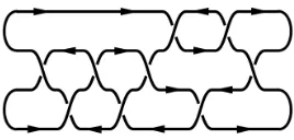
to consider a plat representation of a knot [5, 13]. In this case HOMFLY-PT is provided by the matrix element of a product ofR-matrices or (if we represent complexR-matrices through Racah matrices) product ofR-matrices and Racah matrices. For example, the easiest plat representation, two bridge, is equivalent to a one bit quantum code [12]. Any HOMFLY-PT polynomial in this case is a quantum program. Some random two bridge knot is presented on the Fig. 1.
Figure 1.Typical plat representation for the knot (it is a two-bridge case: there are two arcs at the left and at the
right). This concrete knot is 914in the Rolfsen table [14].
4 Acknowledgements
The work is done in a collaboration with D.Melnikov, A.Mironov, A.Morozov and An.Morozov. The work is supported by the RFBR grant 18-01-00461-a and by joint grant 17-51-50051-YaF. Author thanks the support by the grant of the Foundation for the Advancement of Theoretical Physics and Mathematics "BASIS".
References
[1] M.A. Nielsen and I.L. Chuang, Quantum Computation and Quantum Information, Cambridge University Press, 2000
[2] A.Yu. Kitaev, A.H. Shen and M.N. Vyalyi,Classical and quantum computation, Providence, RI: AMS, American Mathematical Society. xiii, 257 pp. (2002) [Graduate Studies in Mathematics, 47] M. Hayashi, S. Ishizaka, A. Kawachi, G. Kimura and T. Ogawa,Introduction to Quantum Infor-mation Science, Springer, 2015
[3] Ch. Nayak, S.H. Simon, A. Stern, M. Freedman and S.D. Sarma, Rev. Mod. Phys.80(2008) 1083, arXiv:0707.1889
[4] J.W. Alexander, Trans.Amer.Math.Soc.30(2) (1928) 275-306
V.F.R. Jones, Invent.Math.72(1983) 1 Bull.AMS12(1985) 103Ann.Math.126(1987) 335 L. Kauffman,Topology26(1987) 395
P. Freyd, D. Yetter, J. Hoste, W.B.R. Lickorish, K. Millet, A. Ocneanu, Bull. AMS.12(1985) 239 J.H. Przytycki and K.P. Traczyk, Kobe J. Math.4(1987) 115-139 J.H. Conway, Algebraic Proper-ties, In: John Leech (ed.),Computational Problems in Abstract Algebra, Proc. Conf. Oxford, 1967, Pergamon Press, Oxford-New York, 329-358, 1970
[5] E. Witten, Comm.Math.Phys.121(1989) 351-399
[6] L.Kauffman, S.Lomonaco, New Journal of Physics,4(2002) 73.1-18;6(2004) 134.1-40,
quant-ph/0401090
[7] E. Guadagnini, M. Martellini, M. Mintchev, Clausthal 1989, Procs.307-317; Phys.Lett.B235
(1990) 275
[8] A. Mironov, A. Morozov and An. Morozov, JHEP03(2012) 034, arXiv:1112.2654
H. Itoyama, A. Mironov, A. Morozov, An. Morozov, Int.J.Mod.Phys. A27 (2012) 1250099, arXiv:1204.4785
A. Anokhina, A. Mironov, A. Morozov and An. Morozov, Nucl.Phys. B868 (2013) 271-313, arXiv:1207.0279
[9] V. Chari and A. Pressley,A Guide to Quantum Groups, (1994), Cambridge University Press, Cambridge
J. Fuchs,Affine Lie Algebras and Quantum Groups, (1995), Cambridge University Press, Cam-bridge
[10] M. Jimbo, Lett. Math. Phys.10(1985) 63-69
[11] V.E. Korepin, N.M. Bogoliubov and A.G. Izergin,Quantum Inverse Scattering Method and Cor-relation Functions, (1997), Cambridge University Press, Cambridge
[12] D. Melnikov, A. Mironov, S. Mironov, A. Morozov and An. Morozov, Nucl. Phys. B926(2018) 491, arXiv:1703.00431
[13] D.Galakhov, A.Mironov, A.Morozov, JETP, 120 (2015) 549-577 (ZhETF, 147 (2015) 623), arXiv:1410.8482
D. Galakhov, D. Melnikov, A. Mironov and A. Morozov, Nucl.Phys. B899 (2015) 194-228, arXiv:1502.02621