C om putational stu d ies o f th e
electronic stru cture o f tran sition
m etal and p-block com pounds
E va L in n ea F orslu n d
U n iv e r sity C o lleg e L on d on
T h e s is s u b m itte d for t h e d e g r e e o f P h .D . in C h e m is tr y
P ro Q u est Num ber: U 6 4 3 4 4 0
All rights r e serv e d
INFORMATION TO ALL U S E R S
T h e quality o f this reproduction is d e p e n d e n t upon th e quality of th e c o p y su bm itted . In th e unlikely e v e n t that th e author did not s e n d a c o m p le te m an u scrip t
and th ere are m issin g p a g e s , t h e s e will b e n oted . A lso , if m aterial had to be rem oved , a n ote will ind icate th e d eletio n .
uest.
P ro Q u est U 6 4 3 4 4 0
P u b lish ed by P ro Q u est LLC (2016). C opyright o f th e D issertatio n is held by th e Author. All rights r e se r v e d .
This work is p rotected a g a in s t u nau th orized cop yin g under Title 17, United S ta te s C o d e . Microform Edition © P ro Q u est LLC.
P ro Q u est LLC
7 8 9 E a st E ise n h o w e r Parkw ay P.O. B ox 1 3 4 6
A b stract
A series of calculations, using time-dependent density functional theory as imple
mented in the Amsterdam Density Functional (ADF) program, have been carried out
on 2,3-dialkynyl-1,4-diazabuta-1,3-diene palladium molecules and their complexes in
order to determine their electronic excitation energies for comparison with experi
mental UV/Vis absorption spectra. A molecular orbital explanation is presented for
the bathochromic shift which occurs when hydrogen is substituted for a dimethyl
amino-group in the para position of the aryl rings of the free ligands. The near in
frared (NIR) absorption in the free diazabutadiene is found to be a H O M O ^LU M O
transition, and the bathochromic shift was found to be due to a destabilising an
tibonding interaction between the NjVMe2 Pvr and the aryl ring in the HOMO. It was found th at palladium stabilises the LUMO and hence complexation reduces the
HOMO-LUMO gap, causing a further bathochromic shift of the NIR absorption.
The bond energies of the diatomic halogens (F2- ^ l2) have been studied, using
the ADF program, to gain an understanding of why F2 has an unusually low bond energy. The low F-F bond energy was found to be the result of a lower than ex
pected electrostatic energy at the equilibrium bond length. This in tu rn is due to
large electron-electron repulsion of F charge clouds. The gain in the electrostatic
energy th at occurs when the bond length is decreased from equilibrium is, however,
outweighed by the increase in Pauli repulsion energy which is greater in F2 than in
the heavier halogens due to the more rapidly varying orbital overlap.
The potential energy surface of the CIO4-HO2 reaction has been studied using the
ab initio and hybrid-DFT methods. The reaction was found to take place either on a singlet surface to form HCl and O3 via a transition state, or on the triplet surface
to form HOCl and 0 2(^S) without any activation barrier being present. No other
transition state besides the one mentioned above could be found due to a variety
of computational problems. Similar problems occurred when using the Gaussian 98
program, suggesting th at D PT calculations on these type of radical reactions should
A b b reviation s
ADF -Amsterdam Density Functional
AO -Atomic Orbital
BO -Born-Oppenheimer
CCSD(T) -Coupled Cluster with Single, Double and perturbative
Triple excitations
COSMO -Conductor-like Screening Model
DAD -1,4-diazabut a-1,3-diene
DCM -Dichloromethane
DFT -Density Functional Theory
GGA -Generalised Gradient Approximation
CTO -Gaussian-type Orbital
HF -Hartree-Fock
HOMO -Highest Occupied Molecular Orbital
i-Pr (^Pr) -iso-propyl
L -Ligand
LDA -Local Density Approximation
LUMO -Lowest Unoccupied Molecular Orbital
M -Metal
Me -Methyl
MO -Molecular Orbital
NIR -Near Infrared
PDT -Photodynamic therapy
R, R' -Substituents
SCF -Self-Consistent Field
SOC -Spin-Orbit Coupling
STO -Slater-type Orbital
TD-DFT -Time-dependent Density Functional Theory
TDHF -Time-dependent Hartree-Fock
XC - Exchange- Correlat ion
A cknow legem ent
First of all I would like to thank both my supervisors. Dr. Rudiger Faust for giving
me the opportunity to do a PhD at UCL. Dr. Nikolas Kaltsoyannis for introducing
me to the world of computational chemistry and for all your encouragement and
help.
Thanks to Emma O ’Grady for valuable discussions throughout the past few years
and for your help with proofreading this thesis.
Thanks to everyone, past and present, in 019 and 025, and the Faust group for
making the atmosphere so pleasant.
Thanks to the Ohemistry Department for the teaching assistant scholarship.
At last I would like to thank my parents for all their support and encouragement,
C ontents
1 T h eoretical and C om p u tation al C on siderations 1
1.1 Schrodinger E q u a tio n ... 2
1.2 Hartree-Fock A pproxim ation... 3
1.3 History of D F T ... 6
1.4 Exchange-Correlation Functional ... 8
1.5 Basis S e t s ... 11
1.6 Calculating Excitation Energies using Time-Dependent Density Func tional T h e o r y ... 13
1.7 Relativistic E f f e c t s ... 15
1.8 The Amsterdam Density Functional Code ... 18
1.8.1 The Conductor-like Screening Model of S o lv a tio n ... 18
1.8 .2 Ziegler-Rank Energy Decomposition S c h e m e ... 21
1.9 Other Computational Methods ... 22
1.10 Overview of T h e s i s ...23
2 G eneral com p u tation al and exp erim en tal d etails 25 2.1 Computational d e t a i l s ... 25
3 E lectronic T ransition E nergies in 1,4-d icizab u ta-l,3-d ien e C om pounds
and th eir C om plexes w ith P allad iu m 28
3.1 In tro d u c tio n ...28
3.2 Determining the Most Suitable Computational P a r a m e te rs ... 33
3.2.1 Basis S e t ...34
3.2.2 Exchange-Correlation F u n c t i o n a l... 36
3.2.3 Solvent S u r f a c e ...37
3.2.4 C o n clu sio n s... 37
3.3 Comparison of Experimental and Calculated G e o m e tr ie s ... 39
3.3.1 Gas-phase Molecular Geometries ... 39
3.3.2 Molecular Geometry in S o lu tio n ... 40
3.3.3 C o n c lu sio n s... 42
3.4 Electronic Transitions and UV/Vis Spectra of 1,4-diazabuta-1,3-dienes 44 3.4.1 Comparison of the Calculated Electronic Absorption Spec trum of 2 with the Experimentally Determined Spectrum of 1 ...44
3.4.2 Comparison of the Calculated and Experimental Electronic Absorption Spectrum of 1 ... 47
3.4.3 Comparison of the Calculated Electronic Absorption Spec trum of 6 with the Experimentally Determined Spectrum of 5 ...50
3.4.4 Comparison of the Calculated Spectrum of 1 0 with the Ex
perimentally Determined Spectrum of 9 54
3.4.5 Comparison of the Calculated Spectrum of 14 with the Ex
3.4.6 C o n c lu sio n s... 58
3.5 Electronic Transitions and UV /V is Spectra of 1,4-diazabut a-1,3-diene
Palladium (II) c o m p le x e s ... 60
3.5.1 Importance of Exchange-Correlation Functional in Palladium
C om plexes...60
3.5.2 Importance of Basis Set in Palladium Complexes ... 64
3.5.3 Comparison of Experimental and Calculated Geometries of
the Palladium Complexes ...6 6
3.5.4 The Calculated Electronic Structure of 4 and Comparison of
the Calculated Electronic Absorption Spectrum of 4 with the
Experimentally Determined Spectrum of 3 ...67
3.5.5 Comparison of the Calculated Electronic Absorption Spec
trum of 8 with the Experimentally Determined Spectrum of
7 73
3.5.6 Comparison of the Calculated Electronic Absorption Spec
trum of 1 2 with the Experimentally Determined Spectrum of 1 1 ...78
3.5.7 Comparison of the Calculated Electronic Absorption Spec
trum of 16 with the Experimentally Determined Spectrum
of 1 5 ...81
3.5.8 Further Studies of Electronic Excitation Energies in Diaza
butadiene Palladium C om plexes... 84
3.5.9 Solvent Dependence of 7 ... 89
4 T h e S tren gth o f th e X2 Bond; X = F , C l, B r, I 93
4.1 In tro d u c tio n ...93
4.2 Determining the Most Suitable Computational P a r a m e te r s ... 97
4.2.1 Exchange-Correlation F u n c t i o n a l... 97
4.2.2 Basis S e t ... 105
4.2.3 Spin-Orbit C o u p lin g ... 107
4.2.4 C o n clu sio n s... 108
4.3 Population A nalysis... 108
4.4 Energy D e c o m p o sitio n ...110
4.5 C o n c lu sio n s... 117
5 Investigation s o f th e P o ten tia l E n ergy Surface o f th e CIO -f H O2 R eaction 119 5.1 In tro d u c tio n ... 119
5.2 Computational D e t a i l s ...123
5.3 Studies of the Potential Energy Surface using the ADF Program . . . 124
5.3.1 Singlet S u r f a c e ... 124
5.3.2 Triplet Surface ... 129
5.4 Studies of the Potential Energy Surface using the Gaussian 98 Program 131 5.5 C o n c lu sio n s... 133
A P roced u re for th e sy n th esis o f N ,N ’-b is(p h en y l,6 -b is(triiso p ro p y lsily
l)-h ex a -l,5 -d iy n e-3 ,4 -d iim in e palladium dicl)-hloride (com pound 3, cl)-hapter 3 )1 3 4
List o f Figures
1 .1 COSMO s u r f a c e s ...2 0
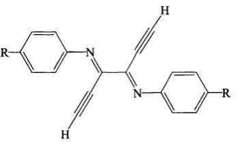
3.1 General structure of the
N,N'-phenyl-2,3-dialkynyl-l,4-diazabuta-l,3-dienes...30
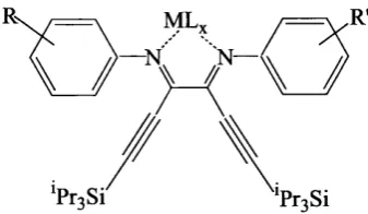
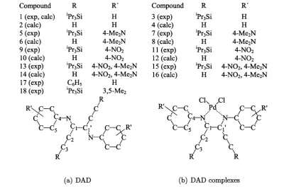
3.2 General structure of the
N,N'-phenyl-2,3-dialkynyl-l,4-diazabuta-l,3-diene metal complexes...31
3.3 Schematic representation of the DAD ligands and corresponding pal
ladium complexes discussed in this s tu d y ...33
3.4 The relative total bonding energy of 2 as a function of the N-Ci-Ci'-N dihedral angle... 41
3.5 The change in transition energies and oscillator strength when gradu
ally changing the C1-N-C4-C5 dihedral angle, i.e. rotation of the aryl
rings... 42
3.6 The relative bond energy of 2 as a function of the C1-N-G4-C5 dihed ral angle... 43
3.7 The experimental UV/Vis absorption spectrum of 1 and the simu
lated spectrum of 2. The intensity of the longest wavelength peak in the simulated spectrum of 2 has been set equal to th a t in 1... 44
3.9 The experimental and simulated UV/Vis absorption spectrum of 1.
The intensity of the longest wavelength peak in the experimental
spectrum has been set equal to th a t in the simulated spectrum. . . . 48
3.10 The experimental UV/Vis absorption spectrum of 5 and the simu lated spectrum of 6. The intensity of the longest wavelength peak in the simulated spectrum of 6 has been set equal to th a t in 5 ...52
3.11 Three-dimensional representation of the HOMO (32b) of 6... 52
3.12 The simulated spectrum of 4 using two different exchange correlation functionals; LDA(VWN) and GGA(BP8 6)...61
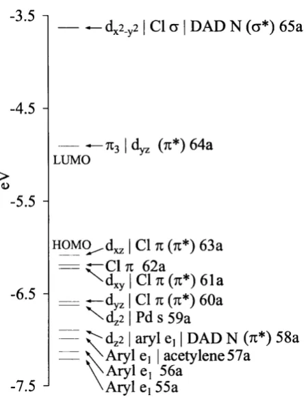
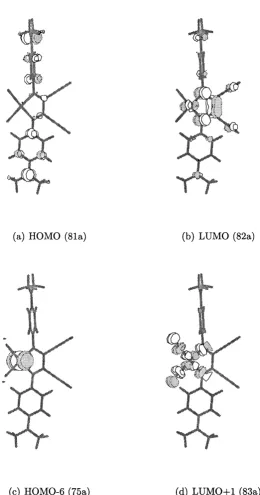
3.13 Molecular orbital energy level diagram for 4 ...6 8 3.14 Three dimensional representations of selected MOs of 4...69
3.15 The experimental UV/Vis absorption spectrum of 3 (solid line) and the simulated spectrum of 4 (dashed line). The intensity of the most intense band in the simulated spectrum of 4 has been set equal to th at of the longest wavelength transition band in 3 ... 71
3.16 Molecular orbital energy level diagram of 8... 75
3.17 The experimental UV/Vis absorption spectrum of 7 (solid line) and the simulated spectrum of 8 (dashed line). The intensity of the longest wavelength peak in 7 has been set equal to th a t of the second longest wavelength peak in the simulated spectrum of 8... 75
3.18 Three dimensional representations of selected MOs of 8...77
3.19 Molecular orbital energy.level diagram for 12... 79
3.20 Molecular orbital energy level diagram for 1 6... 82
3.21 Molecular orbital energy level diagrams for 4 , 8, 12 and 16... 85
3.23 Absorption spectra for 7 in different solvents. The dielectric constant
is given next to the solvent... 89
4.1 Difference between X-only and VWN as the LDA option using two
common GGA functionals and the QZ4P basis set. R ed=B P8 6,
green=PW 91...101
4.2 A selection of calculated bond energies for X2 (X =F, Gl, Br, I) using
different GGA functionals with X-only for the LDA part. Blue=Perdew,
red=PBEc and green=PW 91c...103
4.3 Decomposition of the bond energy, F/, in F2 when changing the F-F
bond distance. £'®'®*^*=electrostatic energy; Pauli repulsion
energy; orbital interaction energy... I l l
4.4 Energy decomposition analysis terms at equilibrium bond distance. . 112
4.5 Pauli repulsion energy (hashed line) and total overlap (solid line) as
a function of change in bond length from reqm... 116
5.1 The energies of the stationary points on the GIG 4- HO2 potential
energy singlet and triplet surface relative to a zero for the reactants,
as obtained at the GGD//GGSD(T) level of theory...125
5.2 Ball and stick representations of the stationary points on the GIG -f
HG2 singlet potential energy surface as obtained at GGD level of theory. 125
5.3 Ball and stick representations of the stationary points on the GIG -H
HG2 singlet potential energy surface...127
5.4 The energies of the stationary points on the GIG -|- HG2 potential
energy surface relative to a zero for the reactants using the BP8 6
5.5 Ball and stick representations of the stationary points on the CIO +
HO2 triplet potential energy surface as obtained at CCSD(T) level of
th e o r y ... 129
5.6 The relative energy as a function of the 01-H distance using m in4
List o f Tables
3.1 Comparison of the effect of different aryl substituents and metals on
the longest wavelength absorption in DCM... 31
3.2 Calculated wavelengths (nm), transition energies (eV) and oscillator
strengths and orbital characteristics of the bands in the UV /V is spec
tra of planar 2 with different basis sets using the LDA...35
3.3 Calculated wavelengths (nm), transition energies (eV) and oscillator
strengths for planar 2 with different exchange-correlation functionals
and the DZP basis set. Transitions with the same MO character (not
given) are grouped together horizontally. ... 36
3.4 Calculated wavelengths (nm), transition energies (eV) and oscillator
strengths for planar 2 with different solvent surfaces using the LDA (VWN)
functional and the DZP basis set. Transitions with the same MO
character are grouped together horizontally... 38
3.5 Selected computational and experimental geometric parameters for
DAD molecules. Bond lengths are given in  and bond/dihedral
angles are given in °. The atom and compound numbering scheme is
3.6 Experimental and calculated wavelengths and energies, and calcu
lated orbital characteristics of the bands in the UV /V is spectra of 1
and 2. All transitions are of symmetry...45
3.7 Experimental and calculated wavelengths and energies, and calcu
lated orbital characteristics of the bands in the UV /V is spectra of 5
and 6. All transitions are of ^A symmetry...50
3.8 Calculated wavelength (nm), energies (eV), oscillator strengths and
excitation coefficients, calculated for 10 and obtained experimentally
for 9. The calculated orbital characteristics are also presented... 57
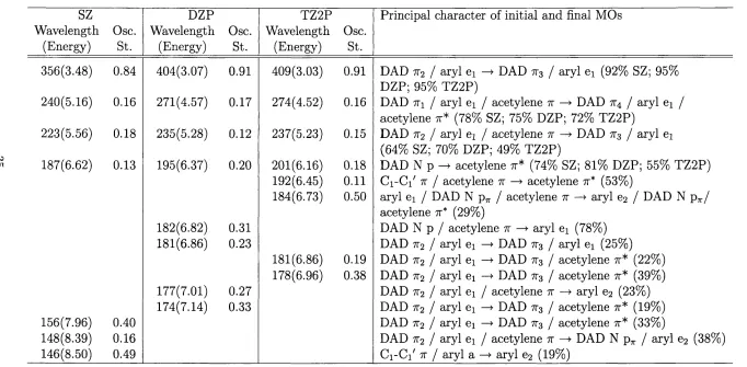
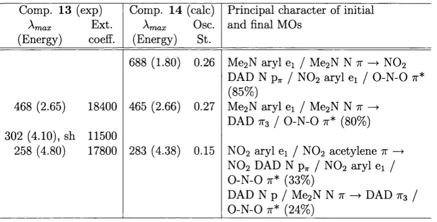
3.9 Calculated wavelength (nm), energies (eV), oscillator strengths and
excitation coefficients, calculated for 14 and obtained experimentally
for 13. The calculated orbital characteristics are also present... 57
3.10 Calculated wavelengths (nm), transition energies (eV) and oscillator
strengths for the band around 400 nm in 4, using different exchange
correlation functionals and rotating the aryl rings around C1-N-C4-C5. 62
3.11 Calculated wavelengths (nm), transition energies (eV) and oscillator
strengths for the band around 400 nm in 4, using different XC-
functionals and with the aryl rings fixed at Ci-N-C4-Cs=62°. The
XC-functional used in the geometry optimisation is given first, fol
lowed by the XC-functional used in the calculation of excitation en
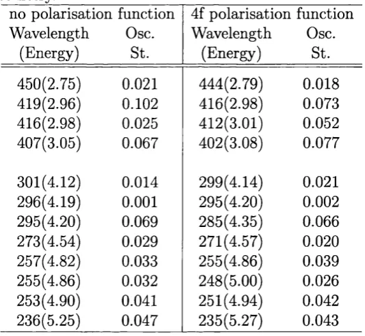
3.12 Calculated wavelengths (nm), transition energies (eV) and oscillator
strengths for 4 at the geometry optimised with and without a 4f polar
isation function in the basis set of palladium. The transition energies
are calculated with the same basis set th a t was used to optimise the
geometry...65
3.13 Selected experimental and computational geometric parameters for
11 and 12 respectively. Bond lengths are given in Â, bond/dihedral
angles are given in °...6 6
3.14 Experimental and calculated wavelengths and energies, and calcu
lated orbital characteristics of the bands in the UV/Vis spectra of
DAD Palladium complexes. Calculated wavelengths and energies
have been modified according to equation 3.1... 71
3.15 Experimental and calculated wavelengths and energies, and calcu
lated orbital characteristics of the bands in the UV/Vis spectra of
DAD Palladium complexes. Calculated wavelengths and energies
have been modified according to equation 3.1... 76
3.16 Wavelength (nm), energies (eV), extinction coefficients and oscillator
strengths, calculated for 1 2 and obtained experimentally for 1 1. The calculated orbital characteristics are also presented... 78
3.17 Wavelength (nm), energies (eV), extinction coefficients and oscillator
strengths, calculated for 16 and obtained experimentally for 15. The
calculated orbital characteristics are also presented... 81
3.18 Calculated wavelength (nm), energies (eV) and oscillator strengths for
3.19 Calculated and experimental wavelength (nm) and energies (eV) for
the low energy transition in 8 in different solvents (adjusted by equa tion 3.1)... 90
4.1 The effect of the London dispersive energy (E'l) on the dissociation energy (Do) of the X2 molecules according to two different studies. Energies in k J/m o l... 94
4.2 Bond energies (kJ/m ol) for the diatomic halogen molecules. No zero
point energies (ZPE) are included unless stated ... 98
4.3 Selection of calculated bond lengths (Â) using different XC-functionals.
X-only was used for the LDA part of the XC-functional...104
4.4 Selection of calculated vibrational frequencies (cm“ ^) using different
XC-functionals. X-only was used for the LDA part of the XC-functional. 105
4.5 Bond energies (kJ/m ol) obtained using different basis sets. No
spin-orbit coupling was included... 106
4.6 Bond lengths, total bonding energies and frequencies calculated using
the X -only/PW 91x/PBEc functional and QZ4P basis set... 109
4.7 % contribution to valence tt^, tt^ and a g MOs. Minimum contribution
1% 110
4.8 Sum of all overlaps in the S'-matrix and the electrostatic energy for
F2, CI2, Br2 and I2 at their equilibrium bond distance... 114
4.9 Optimised bond distance r (Â) and electrostatic energy (kJ/m ol) for
the first three diatomic molecules in the chalcogen series and the
4.10 Energy decomposition of the bond energy (kJ/m ol) for F2 at different
bond distances... 115
C hapter 1
T heoretical and C om p u tation al
C onsiderations
In this thesis three different projects in the field of com putational chemistry are
presented; a study of the electronic transition energies in 1,4-diazabuta-1,3-diene
compounds and their palladium complexes, a bond energy decomposition analysis
of the X2 bond (X =F, Cl, Br or I) and finally a study of the potential energy surface of the CIO + HO2 reaction.
The majority of the calculations in all three studies have been carried out using
Density Functional Theory (DFT) and thus I will start by explaining the theory
behind this methodology and the different DFT applications employed in the works
presented herein. A short introduction to some ab initio methods used will also be given.
DFT is based on the electron density-dependent energy functional in contrast to
most other electronic structure theories which contain the wavefunction dependent
energy functional. Despite this, DFT has many similarities with traditional Hartree-
since in the 1960s when DFT was developed, HF theory was already m ature and so
it made sense to follow a similar route to HF theory. Thus a brief introduction to
HF theory will be given before introducing DFT. Some typical features of D FT will
then be discussed and a description of the Amsterdam Density Functional (ADF)
program will be given together with some of its applications.
1.1
S ch ro d in g er E q u a tio n
The Schrodinger equation can be used to describe any molecular electronic system
and is written as:
(1.1)
where, in atomic units.
-\ N - | M - | N M ry N N -\ M M y y
M indexes the nuclei and N the electrons. The first two terms in H are the kinetic energy of the electrons and the nuclei. The other terms are the potential energy
due to nucleus-electron, electron-electron and nucleus-nucleus interactions. The
Laplacian operator, V^, is the sum of the differential operators
-
dx^''+A+A
dy“^ dz^(1.3)
Since the mass of a nucleus is so much greater than th at of an electron, the nuclei
are essentially stationary compared to the electrons. This leads to a first approxim
ation of the Schrodinger equation called the Born-Oppenheimer approximation. If
the nuclei are in a fixed position their kinetic energy is zero and the potential energy
be w ritten as
- l i V N M Y N N -I
^ = + (1.4)
^ i = l i = l A = l i ^ l j > i ' Ü
and the energy obtained from this Hamiltonian is added together with the potential
energy from the nucleus-nucleus repulsion to obtain the total energy of the system.
To find the most accurate wavefunction all electronic structure theories employ
the Variation principle to some extent. The Variation principle states th at the exact
energy can only be found if the exact wavefunction is used and any other energy is
higher than the real energy, i.e.
W H \ ^ ) > (^ o l^ l^ o ) (1.5)
with ^ 0 being the exact wavefunction.
To find this exact wavefunction, the functional E[^] needs to be minimised by searching through all acceptable V-electron wavefunctions.
Eo = p in \ÿ—►yv = p in (iff |T + ^ —►yv Vm + K e |^ ) (1.6)
An acceptable wavefunction has to be quadratic integrable and continuous every
where. Added to this is the criterion of antisymmetry on interchanging two electrons,
to obey the Pauli exclusion principle.
^ ( f i , ^2,. . ., Xi , X j, . . . , Xn ) = ^2, . . . , X j , f i, . . . , Xn ) (1.7)
1.2
H a rtree-F o ck A p p r o x im a tio n
Since it is virtually impossible to go through all acceptable ^-electron wavefunctions
to find the minimum energy and hence the exact function, a subset is created. To
do this, most wavefunction based quantum chemical methods make use of the HF
The wavefunction can be approximated by a Slater determinant of N one-electron wavefunctions called spin-orbitals or molecular orbitals (MO’s), ÿ (f), where the
columns represent the spin-orbitals and the rows represent the electrons.
^2(^2) . . .
(1.8)
01 (^w) 4>2{^n) . . . (j>N{^N)
The spin-orbitals have to be orthonormal, i.e. they have to be orthogonal in space
and normalised so th at the probability of finding an electron in the orbital is unity.
They can be approximated as a linear combination of atomic orbitals (LCAO) or
basis functions, %,
(1.9) 7= 1
where Cyi is a coefficient and b is the to tal number of functions required to represent 0*. The basis functions will be discussed further in section 1.5. The spin-orbitals
are the only flexible part in the Slater determinant and are therefore the part th at
is varied to obtain the lowest energy of the subset. This is done through the use
of the Lagrangian multipliers, leading ultim ately to the HF equation which may be
written as
/ i0i = £i0i z = 1, 2, . . . , AT (1.1 0) Here the Lagrangian multipliers, e*, can be seen as orbital energies and Koopmans’
theorem states th a t Si is the equal to the negative of the ionization energy, —7^. The Fock operator can be expressed as
1 M y
The first two terms are the kinetic energy of the electron in the z-th spin-orbital
and the potential energy due to electron-nuclei attraction. The last term is the
HF potential which allows the electron-electron repulsion to be accounted for in
an average way by a simple one-electron operator instead of the complicated l / r i2
operator. The HF potential is expressed by
Vhf(^I) = - Kj{xi)) (1.1 2)
j
J is the Coulomb operator and can be seen as the potential an electron in spin-orbital
4>i experiences due to the average charge distribution of an other electron in spin- orbital (f)j. K , the exchange operator, does not have a simple physical interpretation (there is no classical analogue) but arises from the antisymmetry requirement.
To solve the HF equation, one has to use iterative methods. First, a set of basis
functions, Xy &re chosen together with initially guessed coefficients, Cy%. These are used to calculate J and K which in turn are used to determine the Fock operator, / . The Fock operator and the basis functions are then used to solve the determinant
det{Fzy — EiSzy) = 0 (1.13)
where F z y are the elements of the Fock-matrix given by
F z y = i X z \ f O - ) \ X y )
(
1-
14)
and S z y is the overlap m atrix given by
S z y = i X z \ X y )
(
1-
1^)
This will then give values for Si th at can be input into the Roothaan-Hall equation
b
to give new coefficients, c^. This cycle is repeated until neither Si or Cyi are improved compared to the previous cycle. The final coefficients, Cyi are used to obtain which can be used to calculate the total energy of the system. This method is called the
self-consistent field (SCF) method.
1.3
H isto r y o f D F T
D FT dates back to the 1920’s when Thomas and Fermi first suggested th a t the
ground state energy can be expressed in terms of electron density (see ref 1 and ref
erences therein). This has the advantage th a t the density is only dependent on three
spatial variables, independent of the number of electrons in the system, whereas the
wavefunction is dependent on three spatial variables and one spin variable for each
electron in the system.
This Thomas-Fermi model is based on a uniform electron gas, similar to a metal,
in which no exchange and correlation effects are taken into account.
ETF[p{f^] = Z J ^ d r + (1.17)
The kinetic energy is harshly approximated whereas the nucleus-electron and electron-
electron repulsion are treated in a classical way. Thomas and Fermi could not prove
th a t it was physically correct to describe the energy in terms of the electron density,
but it seemed reasonable.
In 1964 Hohenberg and Kohn proved th a t the ground-state electronic energy can
be determined completely by the electron density, p.
E\p]=T\p] + V J j ^ ] + V ^ M (1.18)
interaction energy and Vîie[p] is the nucleus-electron interaction energy. The first the
orem of Hohenberg and Kohn states th at the external potential is a unique functional
of the electron density and since the external potential determines the Hamiltonian,
the ground state is a unique functional of the electron density. Their second theorem
shows the validity of the variation principle for the energy, based on the electron
density instead of the traditional wavefunction. These two theorems became the
basis of modern DFT and Kohn later (1998) shared the Nobel Prize in chemistry
for his contributions to DFT.
Kohn and Sham suggested a few years later th at the total electronic energy of a
system can be written as
^ [ p ] — ^non-int[p] J [ p ] + Ke[p] + E x c [ p ] (1 19)
where the first term represents the kinetic energy of a fictitious system with non
interacting electrons th a t has the same density as the real interacting system, J[p]
accounts for the Coulombic interaction between electrons and Vne is the potential energy due to nucleus-electron interactions. The first three terms of equation 1.19
can be calculated exactly whereas the last term, the Exchange-Correlation energy,
ExcIp] = {T[p\ — T n o n - i n t [ p ] ) + ( ^ e e [ p ] “ J[p\) = ^ c [ p ] + ^ n c l [ p ] ( 1 . 2 0 )
can only be approximated. The non-classical potential energy, E^d, contains the self interaction energy due to the difference between the hypothetical and true kinetic
energy as well as the exchange and the correlation energy, i.e. the non-Coulombic
part of the electron-electron interaction.
Just as for the Hartree-Fock approximation, the variational principle is applied
equation
where the effective potential, Ues, is given by:
^eff( 0 — / 2 + Vxc(^i) — (1.2 2)
The effective potential is chosen such th at the ground state density of interacting
electrons, P o { f ) is
P o { f ) = ' t T , M r , s ) \ ^ (1.23)
i s
The first approximation in DFT comes from the potential due to the exchange-
correlation energy, Vxc- If the exact form of Exc and Vxc (its functional derivative) were known, then DFT would be in principle exact. This contrasts with HF theory
in which the Slater determinant docs not represent the real system but is just an
approximation.
1.4
E x ch a n g e-C o rrela tio n F u n ctio n a l
Since the only term in the Kohn-Sham equation th a t can not be stated exactly is the
exchange-correlation (XC) functional, this is where the emphasis on improvements
must lie. Currently there is no structured way to improve these functionals as there
is no clear way of knowing what works and what doesn’t. However, there are some
general features of successful functionals and they will be discussed here.
It is customary to treat the XC energy as two individual terms, the exchange
term and the correlation term. The basis for the XC-functionals is to view them
as representing a uniform electron gas. This means th at the electrons move on a
N , and the volume, V, are considered to approach infinity and the density, N / V = p,
is constant everywhere. The constant density is far from true in most molecular
systems where the electron density usually changes rapidly, but the uniform electron
gas is the only system for which the exchange and correlation functionals can be
solved exactly or at least to very high accuracy.
The simplest form of XC-functional is the local density approximation (LDA).
The XC energy, can be written as
Ekc^[p] = j p{f)£xc{p{f))dr (1.24)
^ x c(p (0 ) is the XC energy per particle. If the spin is taken into account the XC-
energy is instead given by
E k c ^ \ P a , P i 3 ] = J p ( f ) s x c { P a ( r ^ , P i > { ' > ^ ) d r (1.25)
The exchange part, £x, can be expressed by the Slater X^ exchange Q Q 1/3
gx = (1.26)
O 7T
where a=2/Z corresponds to a uniform electron gas.^
The most widely used functional for the correlation part, 6c, is the functional
developed by Vosko, Wilk and Nusair, which employs an analytical interpolation for
mula.^ This functional, denoted VWN, is often combined with the Slater exchange
functional, S, to give the SVWN XC-functional.
If the information about the density is not only obtained from the density at a
particular point, but also from the changes in density through the gradient, V p{f),
the electron gas is no longer homogenous and changes in the electron density can
Gradient Approximations, GGA, and their general expression can be w ritten as
=
j
/(/5a,P/3, Vpa, Vp/3) (1.27)The number of GGA functionals available is extensive and new functionals are
constantly appearing. However, some of the most commonly used functionals for the
exchange part are Becke’s 1988 functional (B8 8 or just B),^ and Perdew and W ang’s
1986 or 1991 functional (PW8 6x, PW91x).^’® For the correlation part, Perdew and
Wang’s PW91c functional is commonly used as is Lee,Yang and P arr’s (LYP)^"^ and
Per dew’s correlation functionals.^®
The obvious step up from GGA would be to include another variable in the
XG-functionals. This has been done in the so called meta-GGA functionals. These
make use not only of the density and its gradient as in GGA, but also of a third
factor which often is the laplacian, i.e. the kinetic energy density.
^ m e t a - G G A P/?] =
J
f { P a , P p , ^ P a , V p ^ , 7 ^ , 7 /? ) ( 1 - 2 8 )These functionals have the computational setback th at it is difficult to optimise
the geometry due to the XG-potential often being non-local and orbital-dependent.
Instead meta-GGA often acts as a post-GGA method and uses the orbitals determ
ined at the GGA level. This limits the use of meta-GGA functionals and they have
not yet proved popular among users.
Another relatively new approach to the XG-functionals are the so-called hybrid
functionals. These make use of a certain amount of the exact exchange energy th at
can be calculated from the Slater determinant of the HF approach, and apply ap
proximate functionals for the correlation energy and the remaining exchange energy.
traditional XC-functionals. One of the most commonly used hybrid functionals is
the B3LYP functional which uses the BeckeSS exchange and the LYP correlation as
the approximate functionals.^^
1.5
B a sis S e ts
To describe molecular orbitals all ab initio and density functional methods in prac tice rely on the selection of appropriate basis sets. The MOs are thus unknown
functions expanded in a set of known functions (the basis set). A basis set is com
plete (has the best single determinant wavefunction th at can be obtained) if an
infinite number of functions are used, as the unknown MO function can then be
expanded exactly from an infinite set of known functions. This leads to a trade-off
between calculation time and accuracy. Since a complete basis set is impossible in
practice, there will always be an absolute error in the calculated result. Therefore
the primary goal is to make the error as small and consistent as possible. The num
ber of functions needed has to be selected for the user’s requirements, but because
of the absolute errors it is meaningless to compare two molecules calculated with
different basis sets.
The basis functions mainly used in the presented work are Slater Type Orbitals
(STO). These are a collection of atomic orbitals th a t can be written as
0: = NYi^rn{0, (1.29)
where are the spherical harmonic functions where the subscript indicates the
Another commonly used basis set type in electronic structure calculations is the
Gaussian Type Orbital (GTO).
Xc,n.i,n.(r,
e,
y ) = iVYi,„(0, (1.30)GTOs are generally less accurate th an STOs, which better represent ‘real’ atomic
functions, and approximately three times as many GTOs compared to STOs are
required to reach the same level of accuracy. However, integrals involving
dependence (GTOs) are easier to compute than those involving (STOs) because
they are suited for analytical integration and hence GTOs dominate most ab initio
codes. The computational implementation of D FT generally requires numerical
integration for the XG potential and this makes the STOs a more appropriate choice
than GTOs. The ADF code, used extensively in this work, uses STOs as its basis
sets.
Basis sets can have different size and complexities. The larger the number of
functions the more complex the basis set. The minimum number of functions to
describe the electrons of a neutral atom determines the contents of the minimum
basis set. For the first row in the periodic table this means two s-functions (Is, 2s)
and one set of p-functions (2pa,, 2py and 2p^). The first step to improve the basis set
is to double the number of functions leading to the first row element being described
by four s-functions (Is, Is', 2s and 2s') and two set of p-functions (2p and 2p'). This
allows a better description of the electron distribution, especially when the electron
distribution is asymmetric, e.g. in a bond. This double basis set is called double zeta
(DZ) where zeta (() comes from the exponent of the STO basis function. Usually
the core electrons are kept as simple as possible and only the valence electrons are
(TZ), quadruple zeta (QZ) and so on.
Polarisation functions, i.e. higher angular momentum functions, can also be ad
ded. p-orbitals can be used to polarise atoms with valence s-orbitals, d-orbitals
for p-orbitals etc. The higher angular momentum functions make it possible to ac
curately describe fluctuations in the electron distribution around an atom which is
essential in methods th a t include electron correlation. One single polarisation (P),
added to a DZ basis set, forms a double zeta with polarisation (DZP). The next
level is called double polarisation (2P) and so on.
Sometime these basis functions are not accurate enough and diffuse functions
have to be used. Diffuse functions are basis functions with a small exponent and
are needed when it is of importance to describe the valence electrons accurately, i.e.
calculations of anions or excited states or polarisability-dependent properties.
1.6
C a lcu la tin g E x c ita tio n E n erg ies u sin g T im
e-D e p e n d e n t e-D e n s ity F u n ctio n a l T h e o r y
The calculation of excitation energies with D FT is more complex than the calcu
lation of static ground state properties. The Kohn-Sham eigenvalues do not have
any real physical meaning and thus Koopmans’ theorem does not exist in DFT.
One method to calculate the excitation energies from the ground state density is
the ASCF method but this is both time consuming and not very accurate. A re
latively recent development is the time-dependent D FT (TD-DFT), which allows
the user to calculate a wide range of frequency dependent molecular properties such
as van der Waals dispersion coefficients, frequency-dependent polarisabilities and
the most popular uses of TD -D FT is to calculate excitation energies and this will
be described hered^’^^
The range of molecules th a t can be used in TD -D FT calculations is comparable
to those th at can be calculated in the ground state SCF calculations, and linear
scaling techniques have recently been developed to allow even larger molecules to
be calculated using TD-DFT.
The basic equation behind time-dependent methods is the time-dependent Schrod-
inger equation which is given by
È { r , t ) ^ { f , t ) = (1.31)
Extending this to DFT, the Kohn-Sham time-dependent equation is
[ - ^ V - = i ^ 4 > i ( r , t ) (1.32)
where the effective potential, Ueff(r, t) is given by
t ) = Uext(r, t ) + f + uxc(c t ) (1.33)
J T-\o
^ext(^, ^) is the external potential, th at is, the Coulombic field and, if present, any
external field. U xc(cO i® time-dependent XC potential. TD -DFT is, just as
time-independent DFT, built on the direct connection between the density and the
external potential. This was proved by Runge and Cross whose theorem states
th a t the time-dependent density uniquely determines the external potential which
in turn uniquely determines the time-dependent wave function. In contrast to the
time-dependent HF equation which only takes into account the exchange effects,
TD-DFT also includes all correlation effects and thus calculates excitation energies
The excitation energy from the z-th orbital, can be obtained from an eigen
value equation
ÜFi = ui^Fi (1.34)
where Fi is the single determinant of KS orbitals from which the oscillator strengths can be obtained. To begin, the determinant Fi has to be guessed. Q is given by
^iaajbr ~ ^aT^ij^ab^^aa ^icr) T ^ ^ia^iaajbryj{^br ^jr) (1.35)
where a and h refer to unoccupied orbitals whereas i and j refer to occupied orbitals.
(J and r refer to the spin of the electron. 6^^, ôab and S(^r are the Kroneker delta th a t are l i i i = j , a = b, a = T and 0 otherwise. If K is set to zero, the excitation energies are the difference between eigenvalues of occupied and unoccupied orbitals.
This is has proven to be a good approximation and a good initial guess. K is a.
m atrix th at contains and can be divided into the Coulomb part and the XC part.
dfidf2 (1.36)
= J J <(>i<7(n)0a<r(n) X
= j J [<l>ic{ri)<l>ac{ri) X fx h ( fi , r2, bj)ipjr{r2)<PbT{r2)] d f i d f2 (1.37)
/x c is the XC kernel which determines the first-order change in the time-dependent
XC potential due to the applied electric perturbation. In equation 1.37 cj indicates the functional’s frequency dependence and the exchange-correlation part of K is therefore time-dependent.
1.7
R e la tiv is tic E ffects
When a particle of mass, mo, moves with a velocity, i/, the actual relativistic mass, m, is given by the formula:
From this, it can be seen th at a slowly moving particle possesses an actual mass al
most equal to the rest mass whereas a quickly moving particle will have significantly
increased mass.
In atomic units, the velocity of an electron in the Is shell of an atom is approx
imately equal to the atomic number, Z, which makes it clear th at the heavier the
atom is, the greater the relativistic mass increase will be of the electron. Therefore
relativity needs to be included in calculations with heavy atoms to give accurate
results.
The Bohr radius is dependent on the mass through 1/m , so when including
relativistic effects the radius decreases as the atomic number increases. The result
of this is th a t the Is-orbital is contracted. The outer s-orbitals are also somewhat
contracted which has traditionally been explained as arising from the orthogonality
constraint on the orbitals. However, it is now believed th a t the contraction of the
higher valence orbitals is due to mixing in of higher energy orbitals. A more
compact s-orbital results in a more effective screening of the nuclear charge which
in tu rn affects the orbitals with higher angular momentum, p-orbitals are mainly
unaffected but d- and f-orbitals become radially more extended.
To include relativistic effects, the particle has to be described using four coordin
ates, three in space and one in time. The time-dependent Schrodinger equation
contains second-order partial derivatives with respect to x, y and z but first-order with respect to t which is not relativistically correct. To solve this problem Dirac produced an equation which treats all four space-time components as first-order.
—ich — -|- Œy — + j + (3mc^ -\-V{x^y^ z) ^ = (1.39)
be a four-component column vector and thus there are in principle four solutions
to equation 1.39; two giving a positive energy with a solution corresponding to a
particle of mass rUe and charge +e, and two giving a negative energy with a solution corresponding to the same mass as the other two but with charge —e. The two negative energy solutions correspond to the two possible spin states of an electron.
The positive energy states correspond to positronic wave functions, hence Dirac
predicted the existence of the positron, which was discovered a few years later (1932)
by Carl D. Anderson.
To include the entire four component Dirac equation in a study of molecules of a
reasonable size, is practically impossible. It is more common to derive atomic basis
sets using the Dirac equation, and then on a molecular level to use for example
the quasi-relativistic Pauli formalism^^ or the zeroth order regular approximation
(ZORA).i»
The Pauli formalism is based on the approximation th a t E — V 2mc^. How ever, at a certain distance close to the nucleus, this approximation does not hold
due to the electrostatic energy, V, becoming more negative.
The ZORA approach, which usually give more accurate results th an the Pauli
formalism, expands the energy in E/{2mc^ — V) and makes use of the approximation
E <C 2mc^ — V. This holds even close to the nucleus.
As noted above, the Dirac equation directly includes the electron spin, thus
allowing the inclusion of spin-orbit coupling (SOC) in relativistic calculations. SOC
stems from the interaction of an electron’s magnetic moment due to the spin angular
momentum, with the magnetic field th at is generated by its own orbital motion, the
as the nuclear charge increases and decreases as I increases. W hen the spin-orbit coupling is weak the Russell-Saunders coupling scheme can be used but fails for
heavier molecules where the coupling is greater. For those molecules the jj-coupling
is more appropriate.
1.8
T h e A m ste r d a m D e n s ity F u n c tio n a l C o d e
The Amsterdam Density Functional (ADF) package is a Fortran program based on
the Kohn-Sham approach to DFT, and offers a wide range of functionalities such
as geometry optimisation, frequencies, excitation energies etc.^^^^ It is developed
by the Theoretical Chemistry groups of the Vrije University in Amsterdam and
Groningen University, the Netherlands, and University of Calgary, Canada.
ADF uses STOs as basis functions to generate the atoms. The fragment approach
to build up a molecule in ADF will be described in detail in section 1.8.2. ADF
supports many XC-functionals (LDA, GGA and meta-GGA) but since it is a pure
DFT program, no hybrid-DFT functionals are available.
Relativistic effects are offered either through the Pauli formalism or the ZORA
approach (see section 1.7) and solvent effects can be taken into account through the
GOSMO algorithm th at has been implemented via GEPOL93 (see section 1.8.1).^^
1 .8 .1 T h e C o n d u c to r -lik e S c r e e n in g M o d e l o f S o lv a tio n
The computational description of molecules in a vacuum or in the gas-phase th at
has been developed over the past several decades now allows us to carry out cal
culations and make predictions with high accuracy. However, the techniques for
it is greatly desirable to be able to include solvent effects. Many physical properties
alter in a solvent system and it is therefore im portant to be able to calculate these
with just as high an accuracy as for systems in the gas phase.
To accurately describe the solute molecule in a solvent on the molecular scale is
difficult, mainly because of the many solvent molecules around the solute molecule
th a t not only interact with the solute but also with each other. There are a number of
different approaches to describe the solvent/solute system. One such approach uses
a dielectric continuum model, with a dielectric medium as solvent with perm ittivity
£ and with the solute embedded in a cavity. A charge distribution is created at the interface between the solvent and the solute, where the solvent has the opposite
sign of the charge distribution in the solute. One big problem is how to describe
the interactions at the interface. Klamt has developed an algorithm known as the
conductor-like screening model (COSMO) of solvation.^®“^® It aims not only to
describe ellipsoidal or spherical surfaces but any arbitrary surface. To do this the
surface is divided into a number of segments. Each segment possesses a center r^, a
surface area and a charge q^. The solvation energy, E'®, is then given by
^ ^ \ R A - r ^ \ 2 ^ \r^ - r„|
E
+Z A
9nVi,{r)p{r)d'i/i V u
/i Y ""At M
where Za is the nuclear charge at Ra- The solvation energy thus contains contri butions from the nucleus-surface and the surface-surface electrostatic interactions
(given by the first and second term respectively) as well as the electrostatic interac
tions within each segment (given by the third term). The final term represents the
interaction between the electron density, p(r), and a surface in which the surface
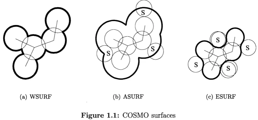
ADF offers four different approaches to construct the surface in COSMO; WSURF,
ASURF, ESURF and K L A M T . W S U R F is the van der Waals surface (see fig
ure 1.1(a)), ASURF is the accessible surface, i.e. the surface generated by the centre
of the solvent molecules rolling on the van der Waals surface (see figure 1.1(b)) and
ESURF is the van der Waals surface th a t is accessible by the solvent molecules with
cusps in the intersecting region (see figure 1.1(c)). KLAMT can be seen as first
creating the ASURF surface and then subtracting the radius of the solvent.
(a) WSURF (b) ASURF
F ig u re 1.1: COSMO surfaces
(c) ESURF
The main concern in a calculation using the COSMO approach is to describe the
surface interactions accurately which makes it im portant to use the correct solvent
radius and van der Waals radius of the solute. Since the solvent is seen as a sphere
in COSMO but in reality the shape of a molecule is often non-spherical, it can be
difficult to choose the right radius. In this study the central carbon atom of the
solvent (usually CH2CI2) was chosen as the centre of the sphere, and the solvent radius was calculated as the distance from the central atom to the atom furthest
away, plus th at atom ’s van der Waals radius. Alternatively, the centre of mass, m
be calculated using:
m i rri2 m*
X : — X x i-H---X 3:2 . . . -I---Xi
m m m
m i m2 , mi , .
y — — X 2/1 H X 2/2 • • • H X y i (1.41)
m m m
m i m2 mi
Z — ---- X Zi -|--- X %2 . . . H---X Zi
m m m
1 .8 .2 Z ieg le r-R a u k E n e r g y D e c o m p o s itio n S c h e m e
ADF defines the molecular bonding energy as the energy difference between the
molecular fragments in their final position and at infinite separation. The com
position of a molecule in ADF starts with two unperturbed fragments or atoms,
with electron density pa and p b, th at are positioned in their final molecular posi tion to give a superposition of fragment densities, Pa + Pb- The interaction energy between these fragments is the traditional electrostatic energy, long in
teratomic distances this energy approaches zero. As the fragments approach each
other the electrostatic energy becomes more negative. This is due to the stabilising
nucleus-electron attraction th a t outweighs the electron-electron repulsion. Accord
ing to general electrostatics and Gauss’ law, the electron-electron repulsion becomes
smaller as the electron clouds begin to interpenetrate. Thus, the bigger the orbital
overlap, the smaller the electron-electron interaction. At very short distances, much
closer than the equilibrium bond distance, the nucleus-nucleus repulsion causes a
significant destabilisation of the electrostatic energy.
The next step is to alter the superposition of electron densities by making sure
th at the antisymmetry constraint (Pauli principle) is followed. The antisymmetry
constraint brings about a reduction in the electron density in the overlap region and
repulsion energy, It should be noted th at the bigger the orbital overlap is,
the bigger the Pauli repulsion will be due to the larger area in which the electron
density is reduced.
The last step allows the electronic wavefunction to relax to self-consistency. This
is done by allowing the virtual orbitals to mix with the occupied orbitals. This has
the opposite effect on the electron density in the overlap region to the antisymmet-
risation in the second step and thus has a stabilising effect on the energy. This
energy is called the orbital interaction energy,
ADF allows for a breakdown of the bond energy into each of these three energies^®
and they are computed using the transition state procedure developed by Ziegler
and Rauk.^^’^^
1.9
O th er C o m p u ta tio n a l M e th o d s
A few other computational methods besides DFT have been employed in this thesis
work; Hartree-Fock (HF), Mpller-Plesset second-order perturbation theory (MP2)
and coupled cluster with single, double and triple excitations (CCSD(T))(for further
information see ref 17).
The HF method has been described in brief in section 1.2. The major disad
vantage of this method is the exclusion of correlation effects th at, for instance, often
results in too low bond energies. The aim of all of the post-HF methods mentioned
is to begin with the HF Slater determinant and to account for electron correlation
from this.
The MP2 method uses the HF wave function as the unperturbed wavefunction
th a t are non-existent in HF. This method usually gives good results in geometry
optimisations and bond energy calculations but a relatively large basis set is required
to get good results and the correlation energy is somewhat overestimated.
The CCSD(T) method has proven very accurate, especially for systems which
can be well-represented by a single Slater determ inant (e.g. molecules with large
HOMO/LUMO gaps). However, the computational cost is significantly higher than
in DFT. All single and double excitation determ inants are calculated whereas the
contributions from the triple excited state are calculated from the formula given
by MP4 and added to the energy. To include all triple excitation determ inants are
too computationally demanding and is only applicable on very small systems. The
double excitations are most im portant to include since they account for most of the
correlation effects.
1.10
O v erv iew o f T h esis
As already mentioned, three projects will be presented in this thesis. First, however,
the computational and experimental details will be described in chapter 2. Following
th at the first project, a study of the electronic transition energies in
1,4-diazazbuta-1,3-diene compounds and their palladium complexes will be presented (chapter 3).
First an introduction to the chemistry of 1,4-diazabuta-1,3-dienes and their metal
complexes will be given, followed by a discussion of the results obtained from this
study. The second project, a bond energy analysis of the X2 bond (X =F, Cl, Br, I),
will then be presented (chapter 4) in the same manner as the previous chapter; first
an introduction and then a discussion of the results obtained in this study. Finally,
C hapter 2
G eneral com p u tation al and
exp erim en tal d etails
2.1
C o m p u ta tio n a l d e ta ils
All calculations have been carried out on Compaq ES40 and Digital Personal Work
station 433au computers using the Amsterdam Density Functional (ADF) program
versions 2.3, 1999, 2000 and 2002 unless otherwise stated.
Molecular orbital plots were generated using the program MOLDEN, written
by G. Schaftenaar of the CAOS/CAMM Centre, Nijmegen, The Netherlands. The
same ’space’ value, 0.05, has been used for all plots. The ADF binary output
files (TAPE21) were converted to MOLDEN format using the program ADFrom99
written by F. M ariotti of the University of Florence.
Slater-type orbital basis sets were employed and their quality was varied as men
tioned in each relevant section. If nothing else is stated, the basis sets were un
contracted, valence only with the frozen core approximation employed; carbon (Is),
corrections were included via the ZORA method where stated. No spin-orbit coup
ling has been taken into account unless otherwise stated. The choice of exchange-
correlation functional is varied as mentioned in each relevant section. The ADF
numerical integration parameters was set to 4 and the energy gradient convergence
criterion was set to 1x1 0“^ au in all geometry optimisations unless otherwise stated. Excitation energies were computed using the time-dependent methods im
plemented in ADF.^^ Solvent effects were included, where stated, using the COSMO
of solvation.
2.2 E x p e r im e n ta l d e ta ils
Although the majority of my work has been computational, I have also done a bit
of experimental work. All reactions were carried out in pre-dried glassware under
nitrogen atmosphere. The reagents were purchased from commercial suppliers and
used without further purification. Solvents were purified and dried according to
customary procedures.^^ Tic was carried out using silica 60 F254 plates (Merck) and the spots were visualised using a UV-lamp.
N,N’-bis(phenyl)-l,6-bis(triisopropylsilyl)-hexa-l,5-diyne-3,4-diimine palladium
dichloride (compound 3, chapter 3) was synthesised as described in appendix A.
The melting point was determined on a Reichert hotstage and is uncorrected.
and NMR spectra were recorded on Bruker AMX400 spectrometer in CDCI3
with residual chloroform (7.24 ppm ^H, 77.00 ppm as an internal reference.
The IR-spectrum was recorded on a Shimadz 8700 FT-IR instrum ent as a KBr disc.
The UV-spectrum was recorded on a Perkin Elmer Lambda 40 spectrometer. The
on a VG ZAB SE machine.
N, N ’-bis (4 ’-dimethylaminophenyl) -1,6-bis (triisopropylsilyl) -hexa-1,5-diyne-3,4-
diimine palladium chloride (compound 7, chapter 3) was synthesised according to
the literature procedures'^ in order to measure the UV-spectra in different solvents
C hapter 3
E lectronic Transition E nergies in
1,4-d iazab u ta-1,3-diene
C om pounds and their C om plexes
w ith P alladium
3.1
In tr o d u c tio n
1,4-diazabuta-1,3-diene (DAD) compounds have many uses, mainly due to the ease
with which their steric and electronic properties can be tuned by changing the
substituents. Synthetically they have applications as building blocks in constructing
4-, 5- and 6-membered heterocycles and in olefin polymerisation.^®
---- N
E-s-cis-E
K.
n— IE-s-trans-E
between the substituents in the 2 and 3 positions. Bulky substituents in the 2 and
3 positions cause steric interactions th a t give rise to the less symmetrical gauche
conformation. It has been found th a t most DADs have a rotational barrier, when
going from the s-trans to the s-cis, ranging from 20 to 28 kJ/mol.^^ This is im portant in their coordination chemistry as the s-cis conformation is needed if the DAD is to act as a chelate.
The DAD has excellent coordination behaviour and can coordinate to a metal
either by its nitrogen lone pairs or by the 7t-C=N.^^’^® It can therefore act as a 2-,
4-, 6- or 8-electron donor in chelating, terminal or bridging arrangements. In its
s-trans conformation it can use only one lone pair at a time to donate two electrons to a metal in the unidentate coordination mode. By rotating around the central
C-C bond to the s-cis conformation, it can use both lone pairs (four electrons) and work as a chelate. It may also act as 6- or 8-electron donor by using one or two
C=N bonds to donate electrons to a second metal but there are few examples of
these and they are not very stable.
The steric and electronic properties of DAD molecules can be tuned by varying
the substituents on the nitrogens or on the central carbons, or by complexation with
a transition metal. Substitution at the 2 and 3 position has been somewhat restricted (to H, Me or fused aryl). However, recently Faust et al have found th at attaching acetylene substituents in these positions not only opens the door to a wider choice