DOI: http://dx.doi.org/10.26483/ijarcs.v8i7.4402
Volume 8, No. 7, July – August 2017
International Journal of Advanced Research in Computer Science
RESEARCH PAPER
Available Online at www.ijarcs.info
ISSN No. 0976-5697
PATH PLANNING TECHNIQUE TO ACHIEVE A DYNAMIC TARGET POINT
Subhadip Boral
Department of Computer Science BarrackporeRastraguruSurendranath CollegeBarrackpore, India
Sudipta Biswas
Department of Computer Science BarrackporeRastraguruSurendranath CollegeBarrackpore, India
Abstract: In this paper a method has been proposed to identify the lowest cost path to reach a destination point from a source point. However, unlike most of the colloquial graph traversal problems, here the destination point is dynamic— not fixed, i.e. changes its position with time. This causes the chaser to update its path planning accordingly, by constantly sensing the position of the destination. During the progression, the chaser may has to side-track many obstacles, for which, in addition to the algorithm for reaching dynamic target through optimal path, two techniques have also been proposed for avoiding obstacles. The proposed method has been compared with the existing techniques for reaching dynamic target such as D*, D* Lite etc. and also with the existing obstacle avoidance techniques such as Bug, NHNA etc., mainly used in Robotics.
Keywords: GIS, Graph Traversal, Dynamic Target, GPS, Obstacle avoidance techniques, NetBeans IDE.
I. INTRODUCTION
In GIS finding shortest (or least cost on the basis of influencing criteria) [3] path between two points plays a very important role. In robotics, in addition to path planning, the robot has to side-track the existing obstacles [1][2][4][5]. Practically the target point may be dynamic also (e.g. to track a pirate ship, to chase a wounded animal adorned with radio collaretc.). During planning for shortest path, existing obstacles should also be avoided. In this proposed method, two obstacle avoidance techniques, namely — Iterative Recovery Method and Shortest Leap Method; have been proposed. Here a number of existing algorithms both for dynamic target search and obstacle avoidance are been studied along with their demerits and the proposed technique tries to overcome them.
II. RELATED WORKS
There exists a number of graph search techniques for finding optimal path to reach a dynamic target. D* [7] is one of them. It splits the search area into suitable sized 8-connected grid world and starts computing the optimal path. This mechanism starts exploring from a particular node and assigns cost to the neighbor 8 nodes and add them in a priority queue based on their cost (costs are additive) and tries to reach goal. As D * is very complex to implement so another technique D* Lite [8] was proposed, which searches back from destination toward source. Lifelong Planning A* or LPA* [10] uses A*, where before exploring a new node future movement cost is updated and decision is taken accordingly.
Obstacles avoidance is a central thing in Robotics as it allows robots to reach its destination avoiding collisions [1][2][4][5]. There are many popular algorithms for the purpose. In Bug 0 Technique, when the robot hits an obstacle it starts following the edge of the obstacle and checks whether the obstacle is avoided or not by imagining a straight line between that point and the goal. In Bug 1 [6], facing an obstacle, the Robot commence its journey along the edge of the obstacle until it reaches the starting point and in this locus, the point with the minimum distance from the destination, is the new journey starting point avoiding obstacle. Bug 2 algorithm [6] creates an incline from the starting point to the goal. After
facing an obstacle, the Robot starts moving by following the boundary of the obstacle and every time generates a new incline from each and every position until the newly generated slope becomes identical to the previous one. The “New Hybrid Navigation Algorithm” [6] is another obstacle avoidance algorithm, which is based on two layers, deliberative layer and reactive layer. These two layers are not dependent to each other. Deliberative layer arranged a reference path on the basis of information that is stored earlier. As well as Reactive layer guide robot independently on the path planed by the deliberative layer. A number of problems observed in the algorithms mentioned here. In Bug 0 algorithm, the direction of journey to avoid the obstacle is chosen arbitrarily, which weakens the method in some cases, particularly when the object is nearer to one end of the obstacle. In Bug 1 the problem may arise when the size of the obstacle is large enough for which the algorithm takes excessive amount of time. In Bug 2, the problem due to biased decision like Bug 0 may arise. Although NHNA technique is beneficial, but it takes a large amount of time to make precise decision. Thus new obstacle avoidance techniques could be proposed to overcome these problems.
III. THE SCHEME
The main motto of the proposed technique is to achieve a dynamic target i.e. a target which changes its position over time, by traversing as shortest distance as possible. Doing so, if it encounters any obstacle in the path, then those obstacles are also efficiently being side-tracked.
Here the works begin with the initial positions of the target and the chaser onto a map containing digitized obstacles.
To meet the objective stated, the scheme could be sub-divided into two broader parts.
1. Methodology to decide the shortest route between the current position of the chaser and the target. It is calculated/determined after each predefined interval of time, as the target point changes its position over time.
Method and Iterative Recovery Method, have been proposed to avoid the obstacles.
The following two sections throws light on Path planning and Obstacle avoidance respectively. Two proposed mechanisms of obstacle avoidance are mentioned in sub sections respectively.below:
Path planning:
To incorporate successful seizing of the target by the chaser some curtailments have been adapted. Firstly, the chaser always has the provision to be familiar with the current position of the target, so that the direction on which the chaser has to move, could be determined accordingly. Next, the movement of the target is self-governing and beyond the control of the proposed algorithm. Thirdly, the speed of the chaser is always greater than the speed of the target.
In real world environment, the position of the target is constantly fetched by using laser gun or GPS device or likewise, however presently to make a simulation of the thing and in order to take a flavour of random dynamic behavior of the target, the following methodology has been incorporated.
Let “a” is the maximum distance which could be travelled by the target per unit time. Obviously the minimum distance traversed in unit time is 0, when the Target has just become still. It can move in any direction also. If the current position of the target is (Xn,Yn) then its next position (Xn+1,Yn+1) is:
Xn+1 = Xn + gcos(α) (1)
Yn+1 = Yn+ gsin(α) (2)
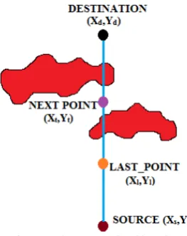
An imaginary straight line is drawn always between the current positions of the source and the destination. Following this path, chaser changes its position in unit time. The chaser senses the target after each unit time and decides its next move. To decide the direction of the next movement, the chaser incorporate the following methodology.
Let, LAST_POINT(XLst,YLst) denotes the coordinate of the current position of the chaser, DESTINATION(Xd,Yd) denotes the coordinates of the current position of the target, r denotes the distance between LAST_POINT (XLst,YLst) and DESTINATION (Xd,Yd), h denotes the distance which can be travelled by the chaser in one unit time, NEXT POINT(Xt,Yt)denotes the point that will be reached (h unit) by chaser towards the destination (i.e. target) after one unit time. In other words, the point with the coordinate (Xt,Yt) is at a distance of h unit from the LAST_POINT(XLst,YLst) and is nearest from DESTINATION (Xd,Yd), which is initially on the straight line , connecting LAST_POINT and DESTINATION.
It is known that, if AB is a straight line connecting two points (x1,y1) and (x2,y2) and P(x,y) is a point lying on the straight line that internally divides the line into two segments with the ratio m:n, then the coordinate of the point P(x,y) could be calculated by using the following formula :
x =((m×x2) + (n×x1))/(m + n) (3)
y =((m×y2) + (n×y1))/(m + n) (4)
Let AB is the connecting edge between LAST_POINT(XLst,YLst) and DESTINATION (Xd,Yd). Let NEXT POINT(Xt,Yt) is the point lying on the straight line which internally divides the straight line into two segments with the ratio of m:n , where m is same as h, i.e. distance traversed in one unit time and n measures the remaining path between LAST_POINT(XLst,YLst) and DESTINATION(Xd,Yd),
which values as (r-h). Then the coordinate of NEXT POINT (Xt,Yt) can be found by incorporating the above formula:
Xt =((h×Xd) + ((r−h)×XLst))/(h + (r−h)) (5)
Yt =((h×Yd) + ((r−h)×YLst))/(h + (r−h)) (6)
By solving the above equations, the coordinate value of NEXT POINT (Xt,Yt) could be found. Special treatment is needed when the next calculated point to reach by the chaser falls within the premises of an obstacle, which is not a legitimate one. The method of Ray-casting is used to determine whether NEXT POINT(Xt,Yt) falls within any obstacle or not. If the NEXT POINT is inside the obstacle, then a point is found which lies on the circumference of the obstacle(polygon). For doing this, a circle is imagined with centre at LAST_PONT(XLst,YLst) and radius h. Let the coordinates of the points constituting the polygon are (x1,y1),(x2,y2). . . .(xn,yn). The constituent points (x1,y1) of the polygon lies on the circle if the following condition satisfied:
(x1–XLst) 2
+ (y1–YLst) 2−
h2 = 0 (7) This checking is done for each and every constituent point of the polygon. Let two intersecting points (M and N) of the circle and the polygon are found. The distance between DESTINATION(Xd,Yd) and each of the two points M and N is now calculated, which possess a lesser distance is regarded as the next destination point. After selecting the legitimate NEXT POINT it is checked, if there exists any more obstacles between LAST POINT and NEXT POINT. For this purpose the slope m between LAST_POINT (XLst,YLst) and NEXT POINT (Xt,Yt) is found.
m = (Yt −YLst)/(Xt −XLst) (8)
[image:2.595.374.506.530.696.2]Next its found that which points of the polygon lie on the edge between the LAST POINT and NEXT POINT. This checking is done for each and every obstacle (digitized polygon). Let z points are found as intersecting points between obstacle (i.e. polygon) and the edge. Among those z points, the point which possess minimum distance from LAST_POINT is denoted as INSC_POINT(Xi,Yi) and the remaining (z-1) points are stored in ascending order depending on the distance from LAST_POINT.
Figure 1: Line Intersecting Obstacles
POINT passes through any obstacle then the method of obstacle avoidance has to invoke.
Obstacle Avoidance Technique:
Let the distance between INSC_POINT and LAST_POINT is d, where 0 < d < h. Thus after traveling d unit along the edge between LAST_POINT and NEXT POINT, the chaser first hits the obstacle at the INSC_POINT. Then any obstacle avoidance scheme has to apply. Two such schemes, namely — Shortest Leap Method and Iterative Recovery Method have been devised here, each with their own merits and demerits. In both of the procedures the idea of driving the search around both of the sides of the obstacle has been included to avoid biased decision and it will always produce shortest path to avoid obstacle in result. Following two sections discuss these methodologies.
A. Shortest Leap Method to avoid Obstacles:
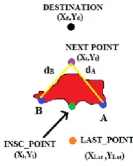
In this obstacle avoidance technique, an idea of two-way search has been incorporated i.e. the mechanism should follow the edge of the obstacle from INSC_POINT in the direction of both left and right for (h-d) unit.
[image:3.595.388.494.114.238.2]In the first unit of time, the mechanism will travel only (h-d) unit because in unit time the chaser can travel h unit and already d unit has been travelled for reaching from LAST_POINT to INSC_POINT, leaving (h-d) unit remaining in that time unit. Incorporating two-way traversal following the edge of the obstacle, it will reach two points, say A and B. Now the distance between DESTINATION to A and DESTINATION to B is calculated. Let the distances be denoted as dA and dB , then point A will be chosen as NEXT POINT iffdA ≤ dB , point B otherwise.
Figure 2: Procedure of Shortest Leap Method
So there will be two conditions that should be considered by the algorithm—
1. As mentioned earlier, the chaser can only travel remaining (h-d) unit in between INSC_POINT and NEXT POINT and will stop after completion of this amount
2. After reaching at the stored INSC_POINT, the INSC_POINT will be sensed as NEXT POINT and way of propagation is calculated again Thus the journey will be propagated from LAST_POINT to INSC_POINT and from INSC_POINT to NEXT POINT. The NEXT POINT will be treated as LAST_POINT in future. The
[image:3.595.105.240.438.606.2]aforesaid procedure can drive the chaser in trounce scenario from where progress towards the target is impeded due to occurrence of a pendulum motion, observed in certain cases. Such a scenario could be explained with the help of following figure (Figure. 3).
Figure 3: Occurrence of Pendulum Motion Criteria
Let at the 1st instance, the target is at the position 1 then the chaser will decide to reach the point m after facing the obstacle. In the 2nd instance, let the target moves to position 2 and the chaser senses point m as INSC_POINT and between m1 and n it will select n as NEXT POINT and move there. In the 3rd instance, if target is at point 3, chaser will select point m again as the NEXT POINT. Thus if the target changes once in the left side and then in the right side of the obstacle, the chaser will also move just like a pendulum, without causing a fruitful result to overcome the obstacle.
To overcome this problem of occurrence of pendulum motion, a particular Threshold value is set (say 5). If the chaser continuously changes its direction, then after reaching the Threshold (i.e. after consecutively changing its direction 5 times), it will stop sensing the Target and without changing its direction furthermore it will just progress to the end of the obstacle to overcome it.
B. Iterative Recovery Method to avoid Obstacles:
There could occur a number of situations where Shortest Leap Method get into such states, from where recovery is very time consuming.
• Situation 1: Possibility of occurrence of pendulum motion from which recovery is time consuming as discussed above (Figure. 3).
• Situation 2: Shortest Leap Method will face another major drawback for a situation when the chaser is inside a circle like obstacle and the target is outside the obstacle, as shown below (Figure. 4), then the chaser will follow the inside edge of the obstacle endlessly and never going to avoid the obstacle, neither announce the failure.
Figure 4: Occurrence of Ceaseless Criteria
[image:3.595.389.525.617.717.2]straight line from each of the points, one after another, on the edge of the obstacle, to DESTINATION. If that particular polygon comes across the straight line, then the algorithm will progress to the next point on the edge of the obstacle until a line connecting a point on the edge of the obstacle and the DESTINATION does not come across that particular polygon but other polygon may come across the connecting path. Suppose from point K connecting line between K and DESTINATION is free of that obstacle then point K will be sensed as new NEXT POINT and this procedure will be triggered from both side of the INSC_POINT and will continue until any of them find the new NEXT POINT or meet each other.
Figure 5: Procedure of Iterative Recovery Method
Following this process one can overcome the ceaseless criteria stated above inside circular obstacle, as both the triggered algorithm meet each other following the inside edge of the circle like obstacle (Figure. 4) so the procedure stops and announces unsuccessful case of obstacle recovery.
IV. IMPLEMENTATION AND RESULTS
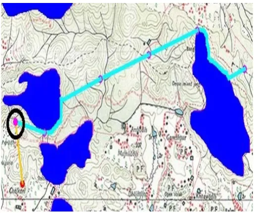
The following Results are found applying the proposed method on the map of Eastern portion of “Giridih” and Northern portion of “Dhanbad”, Jharkhand, India; taken as case study area. The results of enactment, design of GUI and all the required operations have been done using Net Beans IDE 8.0.2 (Java) , which is based on flat -file systems without using databases, hence have increased its portability. The work begins with selection of a map (may be a scanned image or likewise) onto which the obstacles are digitized. Figure 6 demonstrates how the target changes its position randomly and the chaser also updates its path accordingly and finally achieves the target. Here sea-green colored trailing line denotes the movement of the chaser and similarly yellow trailing line is the locus of the target. The locations of the target and chaser are chosen in such a way, that no obstacle avoidance is required.
Figure 6: Method of Dynamic Chasing
Figure 7 demonstrate the avoidance of obstacle using Shortest Leap Method. An idea of occurrence of pendulum motion and its avoidance has also been shown.
Figure 7: Avoiding Obstacle by Shortest Leap Method
Figure 8 demonstrate the avoidance of obstacle using Iterative Recovery Method.
Figure 8: Avoiding Obstacle by Iterative Recovery Method.
V. ANALYSIS AND COMPARISON
O(1)+O(N)+O(ni)+O(N)+O(ni)=O(N)
By keeping both the source and the destination fixed and by increasing the number of obstacles, execution time has measured for both the Iterative Recovery and shortest Leap Method.
[image:5.595.350.534.453.542.2]By varying the number of obstacles from 1 to 8, execution time has measured for both Shortest Leap and Iterative Recovery Method, reflected in Table 1.
Table 1: Performance Analysis for Shortest Leap and Iterative Recovery Method
Number of Obstacles
Time Taken in Milliseconds Shortest Leap
Method
Iterative Recovery Method
1 210 189
2 249 294
3 324 351
4 506 513
5 667 778
6 1220 1061
7 1420 1568
8 1951 2027
Shortest Leap Method senses the target each time during obstacle avoidance also, enabling it to mould its way as per the target’s latest position. It seems quite advantageous to seize the target in a timely manner. However, as discussed earlier, it can fall into a situation of occurrence of Pendulum Motion, where without progressing towards the target it moves around a confined area just like a pendulum. Though the mechanism detects the problem and takes action accordingly but if this criterion arises, the amount of time consumed increases rapidly and give a poor performance.
Another situation forces Shortest Leap Method to perform undesirable steps occurs when the target is practically unreachable i.e. the target or the chaser is surrounded by a group of obstacles which are unavoidable. In this scenario, Shortest Leap Method fails to state the un-reachability and stop and instead of that it goes on processing.
The Iterative Recovery Method works on the principle that when it faces an obstacle it must avoid the obstacle first in direction of the target no matter what are the changes persist in the position of the target in the meantime. This principle makes the method more efficient in case of obstacle avoidance.
There are some situations where Iterative Recovery Method performs unworthy moves. As Iterative Recovery Method performs an obstacle avoiding move in a single step and does not sense the target in the meantime, so it is unable to decide the proper direction of its next move to avoid obstacle. It may be the case that while avoiding the obstacle it has reached to an end of the obstacle, whereas the other end was a much better choice.
Figure 9: Incorporation of wrong direction in Iterative Recovery Method
For example, in the above figure (Fig ure. 9), depending upon the initial position of the target (1), the chaser starts its movement (direction shown by blue arrow), but in the meantime the target changes its position to 2 and then 3, causing to reach the chaser to reach an end, which is far from the target than the other end point.
As compared to Bug 0, Shortest Leap Method senses the obstacle each time; having a probability to search for suitable path to avoid the obstacle quite more often. Iterative Recovery Method although follows somehow almost similar kind of principle but the difference is that it undergoes a two -way tracking, unlike one-way of Bug 0 ; causing to prevent the biased decision taking, as may arise in Bug 0.
In case of Bug 1 [6], the entire obstacle has to traverse first, before getting the way out; which seems to be very time consuming for larger obstacles. But both in Shortest Leap Method and Iterative Recovery Method, they complete their goal (i.e. to avoid the obstacle) even more faster as they sense the obstacle in two way fashion. Even though the obstacle is large, the mechanisms can sense the minimum distant point from the destination in less amount of time and does not have to traverse the total obstacle. In case of Shortest Leap Method, it checks the position of the target in every unit time and decides whether further obstacle avoidance is needed or not and thus makes the mechanism more promising. So the proposed algorithms are less time consuming than the existing one.
In Bug 2 [6], the problem of making biased decision may arise due to the fact that the algorithm tries to avoid the obstacle by making its journey in any arbitrary direction, without any measurement, which may cause sometimes tochoose the wrong one side, making the procedure time consuming one. For example, from the current position indicated by blue circle (Fig. 10), if the particle decides to move towards B, instead of A for avoiding the obstacle, then it is a bad choice; which is possible in Bug 2.
Figure 10: Incorporation of wrong direction in Bug 2 Method
However, both Shortest Leap Method and Iterative Recovery Method make a bi-directional move (i.e. journey towards both A and B) and choose the shortest one path as final, preventing it take any wrong decision. Moreover, Shortest Leap Method always keeps eye on the target to determine whether further avoidance is needed or not and stops making unworthy moves.
Unlike NHA [6], for both of Shortest Leap Method and Iterative Recovery Method, no such reference path is needed to supervise the progress of the robot.
[image:5.595.80.277.647.745.2]unnecessary cell exploration and makes the procedure time consuming.
Though PerSel[11] , a system works in pen-based user interfaces for group selection, provides better result than lasso or rectangle selection, yet when applied for path planning invokes a large set of user interaction in its gestural user interaction. In dynamic goal searching increase in user intervention will result in higher time consumption. In second phrase the system determines linearity coefficient for each and every objects, which is analogous to co-ordinate in GIS, and associated path. PerSel[11] will be excessively time consuming in case of wide ranging target as it will calculate LC for each point and associated path in between target and chaser.
Proposed approach is based on point to pint connection which will be also successful for curvy-linear path like PerSel[11] but will perform better on obstacle avoidance as PerSel need user intervention to select a path to avoid obstacle due to lack of proper intelligence. And this may result in worst-fit path selection.
However, in the proposed method the chaser always routes itself by sensing the target, hence no possibility to move in the opposite way of the target.
VI. CONCLUSION
This work presents a technique to reach a destination in an optimal way, which is dynamic i.e. changes its position over time. During its way it may face some obstacle. The work also presents two methods for avoiding obstacles. There exists a number of techniques both for reaching a dynamic target and for avoiding obstacles. But they have some problems. These problems have been found and tried to overcome in the proposed techniques.
This method could be applied for a number of application areas. It can be used for chasing a GPS enabled car/ boat etc. For biological research purpose, it could be used to chase an animal adorned with radio collar. In this era of automation, it can easily be used to chase something by automated aircraft/ car, where no requirement of manual intervention for avoiding obstacles also required.
VII.ACKNOWLEDGMENT
The authors are thankful to Department of Computer Science, BarrackporeRastraguruSurendranath College, Kolkata-700 120, W.B., India for providing all the infrastructural support to carry out the intended work.
VIII.REFERENCES
[1] M. S. Ganeshmurthy, G. R. Suresh, Path planning algorithm for autonomous mobile robot in dynamic environment, 3rd International Conference on Signal Processing, Communication and Networking (ICSCN), pp 1-6, DOI: 10.1109/ICSCN.2015.7219901, IEEE Conference Publications, March 2015
[2] Luyi Shen et. al., Multi-swarm Optimization with Chaotic Mapping for Dynamic Optimization Problems, , 8th International Symposium on Computational Intelligence and Design (ISCID), pp 132-137, DOI: 10.1109/ISCID.2015.173,IEEE Conference Publications, 2015
[3] M. Gracia et. al., Dynamic Graph-Search algorithm for Global Path Planning in Presence of Hazardous Weather, Journal of Intelligent & Robotic Systems with a special section on Unmanned Systems,Springer Science+ Business Media B.V., 2012
[4] Seohyun Jeon et. al., Cooperative Multi-robot Searching Algorithm, Proceedings of the 12th International Conference - Intelligent Autonomous Systems IAS-12, Volume 2, pp. 749-756, Springer-Verleg Berlin Heidelberg, 2013
[5] Jinpyo Hong et. al, A new mobile robot navigation using a turning point searching algorithm with the consideration of obstacle avoidance, The International Journal of Advanced Manufacturing Technology, Springer-Verleg London Limited, 2010
[6] M. Zohaib, M. Pasha, R. A. Riaz, N. Javaid1, M. Ilahi, R. D. Khan ,Control Strategies for Mobile Robot With Obstacle Avoidance,Journal of Basic and Applied Scientific Research (JBASR) 3 (4), pp.- 1027-1036, 2013
[7] Steven Bell, An Overview of Optimal Graph Search Algorithms for Robot Path Planning in Dynamic or Uncertain Environments , Proceedings of Student Paper Contest, Institute of Electrical and Electronics Engineers Conference, Oklahoma, March, 2010
[8] Sven Koenig ,Maxim Likhachev, D* Lite , Proceeding Eighteenth national conference on Artificia l intelligence, American Association for Artificial Intelligence, pp 476 -483, Menlo Park, CA, USA, 2002
[9] Sven Koenig, Maxim Likhachev, Fast Replanning for Navigation in Unknown Terrain, IEEE Transactions on Robotics (TRO), 21(3), pp. 354-363, 2005
[10] Sven Koenig, Maxim Likhachev, David Furcy, Lifelong Planning A*, Journal Artificial Intelligence, Volume 155 Issue 1-2, pp 93 - 146, Elsevier Science Publishers Ltd. Essex, UK, May 2004