MULTI OBJECTIVE FUZZY SHORTEST PATH SELECTION FOR GREEN ROUTING AND SCHEDULING PROBLEMS

DOI: http://dx.doi.org/10.26483/ijarcs.v8i7.4267

Volume 8, No. 7, July – August 2017

International Journal of Advanced Research in Computer Science

RESEARCH PAPER

Available Online at www.ijarcs.info

ISSN No. 0976-5697

MULTI-OBJECTIVE FUZZY SHORTEST PATH SELECTION FOR GREEN

ROUTING AND SCHEDULING PROBLEMS

Gumpina Vakula Rani

Reasearch Scholar, Dept. of Comp. Sc

Rayalaseema University, Kurnool, AP, India

Dr. Bhaskar Reddy

Professor, Dept. of Comp. Sc

S K University Ananthapur, AP, India

Abstract: The Green Routing and Scheduling Problems deal with the models which relate to ecological issues. For modeling routing and transportation processes characterized by subjectivity, ambiguity, uncertainty and imprecision, fuzzy logic approach happens to be a very promising mathematical approach.The present investigation discusses about the multi objective fuzzy shortest path selection, where the arc lengths are expressed as trapezoidal fuzzy numbers. The shortest paths can be distinguished by using the highest degree of similarity measure. The optimal path selected depends on the different weights given to the MOFSP in the network. The decision maker can select the best one or the most satisfactory solution depending on the priority and nature of the problem. The algorithms are illustrated with a bi-objective optimization problem with crisp and trapezoidal fuzzy values. The numerical experimentation is used to evaluate the proposed model. The experiment results of the proposed model prove that the results lead to the selection of shortest path as a standard algorithm.

Key Words: Fuzzy shortest path, Bellman’s Dynamic Programming, Fuzzy Triangular shortest path, Fuzzy Trapezoidal shortest path, Degree of Similarity, MOSPP(Multi Objective Shortest Path Problem), Green Routing and Scheduling Problems (GRSP).

I. INTRODUCTION

The Green Routing and Scheduling Problems (GRSP) deal with the models which relate to environmental issues. From the last few decades, these problems have been studied by the researchers with great interest. About three-quarters of the oil produced in the world is used for transportation purposes. There is a necessity to conserve and plan for sustainable transportation. The key components to achieve sustainable transportation are effective planning and efficiency of transportation process. Some of the problems like sustainable logistics, waste management [1] etc are dealt by GRSP. Some variants of Green routing and scheduling problems are : (i) the priority based routing, which is considered in public transportation, logistics and waste management, and ii) the time-dependent scheduling of vehicles , which helps to decrease in pollution by avoiding congested routes. Many practical problems may not be characterized by single objective functions completely. In a real time routing network, multiple objectives, for example, scheduling of a vehicle, time, cost, priority, distance, etc. can be assigned to each edge. The task of finding the shortest path with more than one objective is known as the multi-objective shortest path problem. Fuzzy logic could be used successfully to model situations in a highly complex environment where a suitable mathematical model could not be provided [3]. For modeling traffic and transportation processes characterized by subjectivity, ambiguity, uncertainty and imprecision, fuzzy logic approach happens to be a very promising mathematical approach. The use of fuzzy logic is advantageous in several situations especially in decision making processes where the description through algorithms is difficult and the associated criteria are multiplied.

This paper presents the related work in section 2, preliminary definitions and concepts required for

computation and analysis of fuzzy numbers in Section 3. The shortest path algorithms are demonstrated in Section 4. In Section 5, Experiments of these algorithms are conducted and results are compared and presented graphically. Section 6 presents conclusions and provides some pointers for future work.

II.RELATED WORK

Shortest path in fuzzy network was first introduced byauthors [2] in 1980. Floyd's algorithm and Ford’s algorithm was used to find the Shortest path in fuzzy network. Fuzzy shortest path algorithm using Dynamical programming technique was proposed by authors [4]. Authors [5,6,7] proposed Fuzzy shortest path algorithm using linear programming approach. Fuzzy Shortest Path Based on Degree of Similarity was studied by the authors[8,9] . Thus numerous papers have been published on the FSPP. The task of finding Fuzzy Shortest Path using different approaches is discussed and analyzed with a case study.

III. PREREQUISITES

Authors[4] were discussed about the fuzzy- number concepts and definitions in their research work is as follows:

Definition 1: “A fuzzy number is a quantity whose value is

i<j

Authors [12] defined fuzzy- quantity and Fuzzy weighted graphs are as follows :

Definition 2: “A fuzzy quantity is defined as a fuzzy set in the real line R, that is, an R → [0, 1] mapping A. If A is upper semi-continuous, convex, normal, and has bounded support, then it is called a fuzzy number”.

Definition 3:Fuzzy weighted graphs, that is, vertices (or

nodes) and edges (or links) remain crisp, but the edge weights will be fuzzy numbers, as in [6]. A fuzzy weighted graph G=(V,E,

c

) consists of a set V of vertices or nodes vi and a binary relation E of edges ek = (vi,vj) Є VXV; we denote tail(ek) = vi and head(ek) = vj.With each edge (vi,vj) ,

a weight or cost

c

i,j=

c

(vi,vj) = (

c

(vi,vj) 1

,………,

c

(vi,vj)

r

), a vector of fuzzy numbers with r≥1, is associated. Each fuzzy number can be seen as the evaluation of a given criticism.

Definition 4: single objective function: The physical

meaning is that for a single objective function f (x), there is a maximum cost of value M and a minimum cost of value m,and the membership function of objective cost μf(x) is

obtained after being normalized:

μf(x)=













> < < −

−

<

M x f

M x f m m

M m x f

m x f

[image:2.595.324.545.416.534.2]

) ( ... ... ... 1

) ( .

... ... )

(

) ( ... ... ... 0

Objective Shortest Path (MCOP) Problem as follows.

Definition 5: Multi-Objective Shortest Path (MCOP)

Problem Consider a network that is represented by a directed graph G = (V, E) , where V is the set of nodes and E is the set of edges. Each edge (i,j) €E is associated with a primary cost parameter c(i,j) and K additive QoS parameters wk(i,j), k=1,2,3,...K; all parameters are non-negative. Given K constraints ck, .k=1,2...K, the problem is to find a path P from a source node s to a destination node t such that:

def

(i) wk(p) = wk(i,j) = ck for k=1, 2, 3...K,

and def

(ii) c(p) = c(i,j)

is minimized over all feasible paths satisfying

(i)If K=2 an intuitive approximation algorithm based on minimizing a linear combination of the edge weights. More specifically, it returns the best path can be chosen as (ii) S(e) = œ w1(p) + ß w2(p) where œ and ß are the weights and œ , ß € Z+

IV. METHODOLOGY

In this section , a detailed description about the method of analysis is presented which comprises : Shortest Path using

i) Bellman Dynamic Programming for Crisp Arc Lengths(BDPCL) ii) Trapezoidal Fuzzy Shortest Path Length procedure (TFSPL) using DS .

A. Bellman Dynamic Programming for Crisp Arc

Lengths(BDPCL)

Bellman ‘s Dynamic Programming technique is to find the shortest path[13] and can be formulated as follows.

Given a directed graph G = (V, E) with n vertices where V = { v1,v2...vn),vertex 1 is the source and the vertex n is the destination . The shortest path is given by

f(n)=0

f ( i ) = min{di,j + f ( j) │<i, j> Є E}

(1)

Here dijis the edge weight , and f (i) is the length of the

shortest path from vertex ito vertex n .

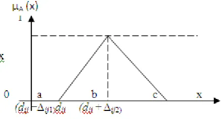
B. Triangular Fuzzy Shortest Path

Fuzzy number A= (a, b, c) is Triangulariff the membership function on R is defined as

μA(x) = (x − a)/(b − a), a≤ x ≤ b (c − x)/(c − b), b≤ x ≤ c

0, otherwise (2)

The edge weight in the network, denoted by dij and the edge weight should be expressed as triangular fuzzy number.

Figure 1: fuzzy number dij

Signed distance from origin to (a, b) = 1/2(a+b). Signed distance between the origin and (a, b, c) is given by

d∗=1/4 (a+2b+c) = dij+1/4 Δij..…….... (3)

If Δij1 = Δij2 , thus the fuzzy problem becomes crisp.

C. Trapezoidal Fuzzy Shortest Path (TFSP)

The membership function (degree) for several points has maximum value which is equal to 1. This gives rise to the trapezoidal shape[10]. Fuzzy number A= (a, b, c, d) is Trapezoidal number iff the membership function on R is defined as

μA(x) = ( x − a)/(b − a), a≤ x ≤ b

1 b≤ x ≤ c

(d − x)/(d − c), c≤ x ≤ d

0 otherwise

[image:3.595.37.284.67.174.2]

DS (d

min

, L

i

)

Figure 2: Trapezoidal fuzzy number

Consider a fuzzy acyclic digraph G = (V,E), where V is the vertices set and E is the edge set. Let the arc length Lijbe the

trapezoidal fuzzy numbers. The trapezoidal fuzzy number changes to the triangular fuzzy number when b = c.

D. Degree of Similarity (DS)

Degree of Similarity is the measurement of the nearness degree of two fuzzy sets. Let dmin(Fuzzy Shortest Length) =

A1 = (a, b, c, d) and Li(ithfuzzy path length) = A2 = (ai, bi,

ci, di) be two Trapezoidal Fuzzy Numbers. If a ≤ ai, b ≤ bi, c

≤ ci, d ≤ dithen the Degree of Similarity (DS) between A1

and A2 can be calculated as follows:

0 if Li∩ dmin= Φ

1/2× (d − ai)2/((d − c) + (bi− ai))

ifLi∩ dmin≠ Φ

wherec< x < d, ai< x < bi

1/2× 1 × [(d − ai) + (c − bi)]

ifLi∩ dmin≠ Φ where bi≤ x ≤ c

…………....(5)

Formulation for DS (dmin, Li) where c < x < d, ai< x < bi.

Let yd be the membership function

yd= (d − x)/(d − c) as c < x < d, ……(5.1)

yd= (x − ai)/(bi – ai) as ai< x < bi .…. ( 5.2)

From (5.1)

yd (d − c) = d − x

x = d + (c − d)yd ...(5.3)

From (5.2) yd (bi – ai) = x −ai

x = (bi −ai)yd + ai …..(5.4)

Equating (5.3) and (5.4)

d + (c − d)yd = (bi – ai) yd + ai[(c − d) − (bi – ai) ]yd = ai− d

height (h )ai – d d − ai

yd = =

(c − d) − (bi− ai ) (d − c) + (bi− ai)

Thus obtain the Intersection Area (IA)

IA = 1/2 × base × height

= 1/2 × (d − ai)2 / (d − c) + (bi− ai)

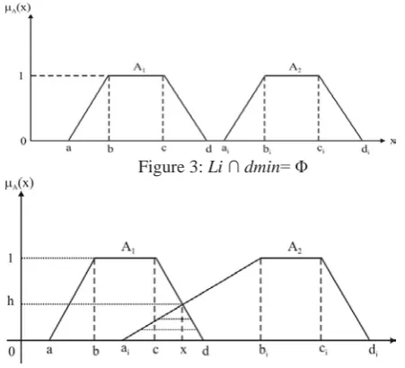
[image:3.595.313.539.110.315.2]

For example, the Degree of Similarity diagrams for two fuzzy numbers represented as Trapezoidal Fuzzy arcs anddmin= X1 and Li = X2 are shown in the figures 3, 4and 5.

Figure 3: Li ∩ dmin= Φ

[image:3.595.316.549.351.470.2]

Figure 4: Li ∩ dmin_= Φ and c < x < d, ai< x < bi

Figure 5: Li ∩ dmin_= Φ and bi ≤ x ≤ c

The similarity degree between the fuzzy shortest length and the individual fuzzy path lengths is considered as the fuzzy similarity measure. The shortest path is the path with the maximum similarity degree.

V.EXPERIMENTS AND RESULTS

In this section , the experiment is carried out to predict the selection of shortest path using i)Crisp values ii) Trapezoidal Fuzzy values. Degree of Similarity is used to determine the rank of Trapezoidal Fuzzy Shortest Paths by considering the network as shown in the figure 6.

A.Bellman Dynamic Programming for Crisp Arc Lengths(BDPCL)

[image:4.595.46.270.57.202.2]

Table 1 : Path Lengths

Figure 6: Network

B. Trapezoidal Fuzzy Shortest Path

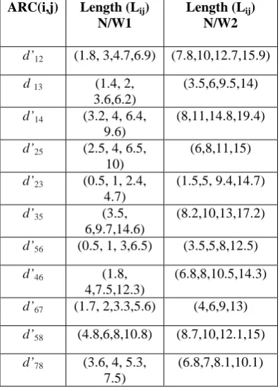
[image:4.595.36.239.307.590.2]

Consider two networks where the arc are represented by trapezoidal fuzzy numbers are presented in the table 2.

Table 2: Trapezoidal Fuzzy Arc Lengths

ARC(i,j) Length (Lij)

N/W1

Length (Lij)

N/W2

d’12 (1.8, 3,4.7,6.9) (7.8,10,12.7,15.9)

d 13 (1.4, 2,

3.6,6.2)

(3.5,6,9.5,14)

d’14 (3.2, 4, 6.4,

9.6)

(8,11,14.8,19.4)

d’25 (2.5, 4, 6.5,

10)

(6,8,11,15)

d’23 (0.5, 1, 2.4,

4.7)

(1.5,5, 9.4,14.7)

d’35 (3.5,

6,9.7,14.6)

(8.2,10,13,17.2)

d’56 (0.5, 1, 3,6.5) (3.5,5,8,12.5)

d’46 (1.8,

4,7.5,12.3)

(6.8,8,10.5,14.3)

d’67 (1.7, 2,3.3,5.6) (4,6,9,13)

d’58 (4.8,6,8,10.8) (8.7,10,12.1,15)

d’78 (3.6, 4, 5.3,

7.5)

(6.8,7,8.1,10.1)

Table 3: Chuang T.N, Kung J.Y, 2005 proposed the algorithm for FSP in their work [8] is as follows :

[image:4.595.310.555.500.707.2]

All the possible paths and the corresponding trapezoidal fuzzy path lengths and the Fuzzy Shortest Length(FSL) are computed by using Algorithm-1 and presented in Table4 and Table5.

Table 4: The Trapezoidal paths Lengths

Path N/W1 (Li) N/W2(Ti)

P1: 1 − 2− 5−8 (9.1,13,19.2,27. 7)

(22.5,28,35.8,45. 9)

P2 : 1 − 3− 5 − 8 (9.7,14,21.3,31. 6)

(20.4,26,34.6,46.

2)

P3 : 1 − 4− 6 − 7– 8

(10.3,14,22.5,35 .4)

(25.6,32,42.4,56. 8) P4 : 1− 3−5−6–

7− 8

(10.8,15,24.8,40

.2) (26,34,47.6,66.8) P5 :1 − 2− 5 −

6– 7 – 8

(10.2,14,21.7,37 .3)

(28.1,36,48.8,66. 5)

P6 : 1 − 2− 3− 5– 8

(10.6,16,24.8,37 )

(26.2,35,47.2,62. 8)

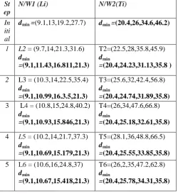
The computational procedure to find the fuzzy shortest length Lmin and the shortest path needed to traverse from source node s to destination node d is presented in table-5.

Table5: The Computational Procedure is as follows:

Input: Li= (ai’,bi’,ci’,di’), where 1<=i<=n Li denotes trapezoidal fuzzy length.

Output:dmin=(a,b,c,d) & denotes the FSL.

Step-1: U={x/x =Li in increasing orders of bi’ & ci’}. U={U1,U2,….,Un} where

Ui= (ai’,bi’,ci’,di’), 1<=i<=n

Step-2:dmin=(a,b,c,d)& U1 = (a1’,b1’,c1’,d1’)

Step-3: Assign i=2

Step-4: Calculate (a,b,c,d) a = min(a,ai‘)

b=     > + − + × − × < ' ) ' ( ) ' ( ) ' ( ) ' ( i a b i a a i b b i a a i b b i a b b c=     > + − + × − × < ' ) ' ( ) ' ( ) ' ( ) ' ( i b c i b b i c c i b b i c c i b c c

d = min (d , ci‘)

Step-5:Assigndmin=(a,b,c,d) and Increment i by 1 Step-6:i< n+1 goto Step 4

Step-7: Compute FSL and Identify the SP with the

St ep

N/W1 (Li) N/W2(Ti)

In iti al

dmin =(9.1,13,19.2,27.7) dmin =(20.4,26,34.6,46.2)

1 L2 = (9.7,14,21.3,31.6) dmin

=(9.1,11.43,16.811,21.3)

T2=(22.5,28,35.8,45.9) dmin

=(20.4,24.23,31.13,35.8 )

2 L3 = (10.3,14,22.5,35.4) dmin

=(9.1,10.99,16.3.5,21.3)

T3=(25.6,32,42.4,56.8) dmin

=(20.4,24.74,31.89,35.8) 3 L4 = (10.8,15,24.8,40.2)

dmin

=(9.1,10.93,15.846,21.3)

T4=(26,34,47.6,66.8) dmin

=(20.4,25.18,32.61,35.8)

4 L5 = (10.2,14,21.7,37.3) dmin

=(9.1,10.69,15.179,21.3)

T5=(28.1,36,48.8,66.5) dmin

=(20.4,25.55,33.85,35.8)

5 L6 = (10.6,16,24.8,37)

dmin

=(9.1,10.67,15.418,21.3)

T6=(26,2,35,47.2,62.8) dmin

=(20.4,25.78,34.31,35.8)

VI. RESULTS

[image:5.595.31.282.55.332.2]

The shortest path selection can be done by using Degree of Similarity (eqn.5). The Decision Makers can choose the preferable alternative paths based on the path ranking. The Similarity Degree measure is calculated between FSL and Li, where ‘ i’ takes the values 1 to 6 and presented for the two networks in the Table 6.

Table 6 : Results of TFSPL using DS

Paths N/W

1 (DS)

Ran k N/ W1

N/W2 (DS)

Ran k N/ W2

P1:1 − 2− 5−8 9.563 1 12.653 2

P2:1 − 3− 5 – 8 6.607 2 16.724 1

P3:1 − 4−6– 7– 8

6.313 4 6.593 3

P4:

1−3−5−6−7−8

5.467 5 5.06 4

P5:

1−2−5−6−7−8

6.362 3 2.997 6

P6:

1−2−3−5−8

5.074 6 4.659 5

The shortest path selection will be done on a fuzzy network with the help of ranking function . The Decision Maker can have choice to the various alternative paths from the list. The rank of the MOSP can be computed by varying the weights of œ and ß in the following equation . Ri the normalized rank function of paths of ith network,

R(pi) = œ R1(pi) + ß R2(pi)

The weighting coefficients œ and ß are assigned to the two objectives respectively. The values œ and ß can take part in the task of priority levels in path selection.

The Rank comparison graph of different approaches i)Crisp Arc Lengths, ii) Trapezoidal Fuzzy Arc Lengths for Shortest Path selection is presented in figure 7& 8 .

BDPCL

Figure :7 – Ranks VS Paths

[image:5.595.317.560.177.639.2]

TFSP

Figure :8 – Ranks VS Paths

The shortest path selection will be done using degree of similarity and the Decision Maker can choose alternative paths with the help of rank given to the paths.The Rank comparison graph of different approaches i)Crisp Arc Lengths, ii) Trapezoidal Fuzzy Arc Lengths for Shortest Path selection is presented in figure 7 and 8. The proposed method solves the GRSP problems very effectively. However, different techniques results in a different solutions

[image:5.595.44.270.442.674.2]

of a problem. In particular, comparing the results obtained in tables 1 and table 5, we may infer that, when the fuzzification method is used, the TFSL and BDCPL techniques provide similar results (figure 7 and 8) with the same set of weights. Also they even rank them in an identical order and which proves that fuzzy multiobjective optimization is quite tolerant of the particular technique .

VII. CONCLUSION

The study of Green Routing and Scheduling problems is gaining momentum in recent years. Shortest paths are computed by expressing the edge Cost as i) Crisp Values ii) Trapezoidal Fuzzy Values. Multi Objective Fuzzy Shortest path Lengths are computed and degree of similarity is used to determine the shortest path selection. The weights of œ and ß are adjusted in such a way that the priority of objective function. The Decision Maker can choose alternative paths with the help of rank given to the paths. Prioritizing the scheduling and the selection of the paths automatically results in the reduction in exhaust fumes facilitates Green routing. The experimental results of this method shows the effectiveness in selecting the shortest path in network design problems and the decision makers further carry out evaluation and validation. Also this method reduces the complexity of solving shortest path in a network.It is observed that shortest path length in Bellman method is same/nearly same with the optimal value in the Multi Objective Trapezoidal Fuzzy Shortest path method. This new approach which is presented can be generalized to n-objective network problem. Finally, it is concluded that the results of the present investigation would provide an excellent platform for making effective and efficient decisions in the case Green Routing and Scheduling Problems and also to design efficient plans for sustainable transportation.

VII. REFERENCES

1. Nora Touati-Moungla and Vincent Jost “On green routing and scheduling problem” hal-00674437, version 1 - 7 Mar 2012. 2. Dubois, D. and H. Prade, Theory and Applications: Fuzzy

Sets and Systems, Academic Press, New York (1980). 3. D. Dubois and H. Prade, 1983, ‘Ranking fuzy numbers in the

setting of possiblity theory,’ Information Sciences, 30, 183-224.

4. Klein, C. M. Fuzzy Shortest Paths, Fuzzy Sets and Systems 39, 27–41(1991)

5. Lin, K. and M. Chen.. The Fuzzy Shortest Path Problem and its Most Vital Arcs, Fuzzy Sets and Systems 58, 343– 353(1994).

6. Okada, S. and T. Soper, “A shortest path problem on a network with fuzzy arc lengths,” Fuzzy Sets and Systems, 109, 129-140 (2000).

7. Yao, J. S. and Lin, F. T. (2003). Fuzzy shortest-path network problems with unce -rtain edge weights, Journal of

Information Science and Engineering, 19, 329-351.

8. Chuang T.N, Kung J.Y, 2005 .The fuzzy shortest path length and the corresponding shortest path in a network, Computers and Operations Research 32 , 1409–1428.

9. P.K.De and Amita Bhinchar ’Computation of Shortest Path in a Fuzzy Network: Case Study with Rajasthan Roadways Network’ International Journal of Computer Applications (0975 – 8887)Volume 11– No.12, December 2010.

10. L. Sujatha and S. Elizabeth “ Fuzzy Shortest Path Problem Based on Index Ranking” Journal of Mathematics Research Vol. 3, No. 4; November 2011.

11.

fuzzy TOPSIS approach for group multi-criteria supplier selection problem Journal of 507–519.

12. Chris Cornelis, Peter De Kesel and Etienne E. Kerre “Shortest paths in fuzzy weighted graphs” international Journal 1068, 2004