Tie-System Calibration for the Experimental Setup of Large Deployable Reflectors

Tie-system calibration for the experimental setup of

large deployable reflectors

A. Cammarata1* , R. Sinatra1, R. Rigato2and P.D. Maddio1

1 _{University of Catania; [email protected]; [email protected]; [email protected]}

2 _{Thales Alenia Space Italia; [email protected]}

* Correspondence: [email protected]; Tel.: +39-095-738-2403

Version March 12, 2019 submitted to Preprints

Abstract:The tradeoff between the design phase and the experimental setup is crucial to satisfy the 1

accuracy requirement of Large Deployable Reflectors. Manufacturing errors and tolerances change 2

the RMS of the reflecting surface and require careful calibration of the tie rod system to be able 3

to fit into the initial design specifications. To give a possible solution to this problem, here two 4

calibration methods, respectively for rigid and flexible ring truss support, are described. Starting 5

from the acquired experimental data on the net nodal coordinates, the initial problem of satisfying 6

the static equilibrium at the measured configuration is described. Then, two constrained optimization 7

problems, for rigid and flexible ring truss support, are defined to meet RMS accuracy of the reflecting 8

surface modifying the tie lengths. Finally, a case study to demonstrate the validity of the proposed 9

methods is presented. 10

Keywords:large deployable reflector; tie adjustment; experimental setup 11

1. Introduction 12

In recent decades, satellite communications have been increasingly spread thanks to the possibility 13

of having high transmitting capacities at a relatively low cost compared to the establishment of a 14

terrestrial broadcasting network. The deployable reflectors represent the most widely used type of 15

structure because of their features such as large scale, high packaging efficiency, high accuracy and 16

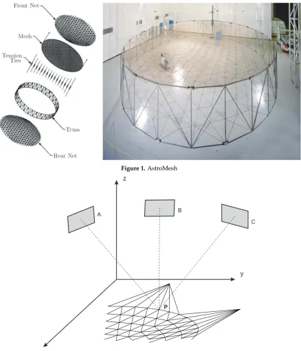
lightweight. Typically, its architecture consists of a deployable ring truss support, two cable nets, facing 17

each other and linked by a series of tension ties, and an RF mesh attached to the backside of the front 18

net. The most representative kind of this type of reflector is the AstroMesh [1], and its components are 19

shown in Fig.1. The electromagnetic performance of these antennas is closely related to the shape of 20

the reflector surface. In turn, this depends on the position of nodes located on the front net. Therefore, 21

it is clear how the measurement process of 3D node coordinates is to be made with extreme accuracy 22

so as to avoid invalidating the real root mean square (RMS) value. 23

In recent years several measurement systems have been developed depending on the application 24

area. Generally, they can be summarised in three categories: 25

• Photogrammetry 26

• Laser tracker 27

• Laser radar 28

The photogrammetry is a measurement technique that uses two-dimensional images of an object 29

to obtain its dimensions. As depicted in Fig.2the photogrammetry is based exclusively on angle 30

measurements: three-dimensional coordinates are calculated via optical triangulation (orintersection) 31

of two or more images taken from different positions. The object to be measured is identified by 32

targets mounted on it, usually made of reflective material so as to produce high contrast between the 33

target and the background [2]. Typically, a calibrated scale bar is integrated into the object in order 34

to reproduce it in true scale. At the end of measurements, a dedicated software calculates the 3D 35

coordinates into the chosen Cartesian coordinate system (x,y,z). 36

Figure 1.AstroMesh

B

C A

P

x

y z

Figure 2.Photogrammetry

Laser tracker and laser radar, instead, are measurement systems based on the estimation of two 37

angles and one length, as shown in Fig.3. Two high-resolution encoders measure the azimuth (θ) and 38

elevation (ϕ) angles, whereas the radial coordinate (r) relative to the center of the target is measured 39

by means of optical interference [3]. Several types of target can be mounted, but the most widely used 40

is the spherically mounted retroreflector (SMR). Differently from laser tracker, laser radar does not 41

require a retroreflector. As a matter of fact, it is capable of measuring the surface of the object with just 42

1% of the reflected signal [4]. 43

Each of these measurement systems, however, has advantages and disadvantages, which need 44

to be assessed on the basis of various factors. Van Gestelet al. [4] identify the influencing factors to 45

P

x y z

t ps

r

Figure 3.Laser tracker

environmental restrictions. Regarding task requirements, the main element to be considered when 47

measuring the position of nodes is the accuracy, since the permissible RMS error on the reflecting 48

surface is less than 1 (mm). Whilst the laser tracker has errors on the order of 1µm, it is too costly due to 49

the high price of each SMR and given the number of nodes (at least a hundred). The photogrammetry 50

turns out to be the best choice [5,6], considering the affordable cost and accuracy of the measure. 51

Furthermore, the possibility of obtaining multiple images from different angles makes it possible to 52

overcome the lower accuracy of the angular encoders of laser trackers. 53

The acquisition of node coordinates is essential for the next calibration step in order to meet the 54

RMS design requirements of the reflecting surface. Generally, the main strategies followed by LDR 55

developers and designers is to use the tie system, connecting front and rear nets, to locally move 56

single nodes. This operation is long and delicate but allows to adjust different error sources such as 57

manufacturing errors [7–9], material definition errors, clearance [10,11], friction [12,13], hysteresis [14], 58

mechanical vibrations [15,16], not perfect behaviour of elastic properties of components. This paper 59

describes a method for the tie system calibration of LDRs with rigid or flexible ring truss. To our 60

knowledge this topic has not been deeply investigated in the literature and the adjustment phase is 61

entrusted with proprietary solutions of LDR companies. The outline of this paper is as follows. In 62

Section2the problem of correcting the parameters to satisfy the static equilibrium in the deployed 63

configuration is first addressed. Then, the method to find the necessary corrections to the tie-system 64

is discussed for the two cases of LDR with rigid and flexible ring truss. In Section3the method 65

is applied to a LDR with asymmetric ring truss developed by Thales Alenia Space. A simulated 66

error distribution is superimposed to the design configuration to represent a real experimental test. 67

Tie-system corrections, expressed in terms of length elongation or shortening, necessary to meet RMS 68

design requirement are obtained for both rigid and flexible ring truss cases. Finally, conclusions close 69

the paper. 70

2. Experimental setting for calibration 71

Once the antenna has been manufactured, it is necessary to carry out some experimental tests 72

in order to check for the RMS of the reflector in the deployed configuration. To do this, the first 73

operation consists of measuring the position of all nodes of the nets with respect to a reference system 74

through one of the methods described in the Introduction. Due to different sources of errors such as 75

manufacturing errors, assembly errors, the deployed configuration will be different from the design 76

operation of the nodes coordinates will be affected by errors. Laser trackers and photogrammetry have 78

errors on the order of 1µm; while laser radar reaches 0.1µm. Anyway, errors related to measurement 79

systems maintain significantly below the proceeding mechanical errors. In the following, two methods 80

for the experimental setting of the rigid and flexible ring truss support are described. 81

Several experimental methodologies [17–20] based on multibody approach have been developed 82

[21–29]. Recently, methods based on the Fuzzy logic [30–34], neural networks [35] and genetic 83

algorithm have been applied for the tensioning of space trusses [36,37]. The proposed methods 84

act on the tensioning system of the ties to fix the errors coming from the construction of the antenna. 85

2.1. Rigid ring truss support: construction length determination 86

Tie cables regulation is usually independent from the actuators used for the LDA deployment [38–40] and from the control system [41–44]. Here, the method to regulate tie cables tension of an antenna with rigid ring truss support is first described. Once the deployment has been carried out and all node coordinates of the net have been measured the reflective surface deviated from the design configuration due to mechanical errors. As a consequence of this deviation, the system of equilibrium equation is not satisfied for the current configuration. Then, denoting withEij,Aij,Lij,L0ij the Young modulus, the cross-section area, the measured length, the construction length of cable/tieij, respectively and withkijthe spring constant of tieij, the system of nonlinear equations for each free nodei, withjadjacent nodes, is not satisfied:

        

       

∑ j

[EijAij L_ij−L0

ij L0

ij

+kij(Lij−L0ij)] xi−xj

Lij 6=0

∑ j

[EijAijLij−L

0

ij L0

ij

+kij(Lij−L0_ij)]yi_L−yj

ij 6=0

∑ j

[EijAijLij−L

0

ij

L0_ij +kij(Lij−L 0 ij)]

zi−zj L_ij 6=0

(1)

wherexl,yl andzl are the measured Cartesian coordinates of thel-th node. It is noteworthy to remark 87

that the only measured parameters are the node coordinates; while themeasuredlength is derived 88

using the Euclidian norm. The remaining parameters of the previous system are design parameters 89

instead, each affected by different types of error. Here, we choose to gather all these errors inside the 90

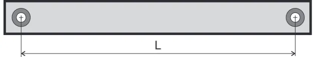
construction lengthL0_ijdefined as the distance between the centers of the eyeletsiandjbelonging to 91

the same cable, as shown in Fig.4. This choice is motivated by the fact that the construction length of 92

the cables is affected by two main sources of errors such as themanufacturing errors, generated during 93

the cutting operation of CNC machines [45], and theassembly errors, coming from a bad placement of 94

the eyelets necessary to connect two or more cables. In order to restore the equilibrium condition in 95

system (1) only the design parameters can be adjusted while the measured parameters describe the 96

real configuration of equilibrium: the measured configuration is already of equilibrium, thus system 97

(1) is to be satisfied in this configuration without changing node coordinates. 98

L

Figure 4.Layout of a cable: the construction lengthL0is affected bymanufacturing errors, generated

during the cutting operation andassembly errorscoming from a bad placement of the eyelets necessary to connect two or more cables

fmincon by giving a constant objective function and setting the eq.(1) as the nonlinear equality constraint, in addition to the linear inequality constraint Lij ≥ L0ij. The resulting constrained optimization problem is described below:

  

 

find L0

ij,∀cables and ties

min constant objective function

s.t. Lij≥L0ij

(2)

Hence, a first check is required. Because the springs used in tension ties require a prestress value, here denoted withF0, representing the minimum value necessary for their activation, the conditionFij≥F_ij0 for each tension tie cable must be verified, where

Fij=kij(Lij−L0ij) (3)

is the spring force of tieij. If the condition is satisfied the next step can be conducted, otherwise the 99

spring belonging to the tie which has failed the test must be replaced and the algorithm starts again 100

calculating the arrayL0of all construction lengths. 101

2.2. Rear nodes determination 102

In the event that only the coordinates of the nodes of the front net are known by measurement, 103

before implementing the algorithm described above, the rear nodes coordinates have to be estimated. 104

Their coordinates are initialized with the design data and the system (1) for each free node of the front 105

and rear net is implemented. It can be noted the dualism between the two methods: in the former, the 106

unknowns are the construction lengths, in the latter the rear node coordinates. Then, the construction 107

lengths are obtained as a consequence using the Euclidian norm. We checked that both methods lead 108

to the same results, unless negligible errors, if the experimental configuration is not too distant from 109

the design one. 110

2.3. Rigid ring truss support: tie calibration 111

Once the configuration satisfying the static equilibrium has been found, the algorithm continues 112

with the estimation of the values of stretching or shortening for each tension tie cable that ensure that 113

the surface accuracy of the reflector can be met. The Figure5shows the screw adjustment system of a 114

tie. One fixed part is connected to a node of the front net while one mobile part, adjustable through a 115

screw, is connected to a node of the rear net. Now, the system of nonlinear equation of each free nodei 116

can be written as follows: 117

        

       

∑ j

[EijAijLij−L

0

ij

L0_ij +kij(Lij−L 0

ij+δLij)] xi−xj

L_ij =0

∑ j

[EijAij Lij−L0ij

L0

ij

+kij(Lij−L0ij+δLij)] y_i−y_j

Lij =0

∑ j

[EijAij L_ij−L0

ij L0

ij

+kij(Lij−L0ij+δLij)] zi−zj

Lij =0

(4)

This system is similar to (1), used to determine the vectorL0, with the difference that, this time, the variables to be found are the stretching/shortening valuesδLijand the coordinates of the free nodes of the front and rear net. The valuesδLijcan be positive or negative: here we assume positive values for tie shortening and negative for tie stretching. Also this system is subject to some constraints. One condition for all net cables is thatL≥L0. For the tension tie cables, for which the valuesδLijare to be considered, the constraint condition is that the final forceFijmust be of traction:

L

k

L

L

L

k

L

L’=L- L

d

d

L

F

F

F’ = F + k

d

L

F = F + k

d

L

Figure 5.Screw adjustment tie system: (left) tie system before the adjustment; (right) tie system after the screw regulation.

Finally, the third constraint is related to the surface accuracy since the RMS error must be lower than 118

the desired design valueRMStarget. This is a typical constrained optimization problem largely used in 119

design optimization of complex systems [46–49] and mechanisms [50–52]. The optimization problem 120

can be summarised as follows: 121

      

     

find x1,y1,z1andδL

min constant objective function

s.t. Lij≥L0ij net cables

Lij+δLij≥L0_ij tension tie cables

RMS≤RMStarget reflecting surface requirement

(6)

wherex1,y1andz1are the free node coordinates andδLis the array containing all correctionsδLij. 122

The RMS is calculated by measuring the minimum distance of the free nodes of the front net compared 123

to the ideal surface of the paraboloid (citazione primo articolo). The initial condition for the free nodes 124

is represented by their experimental measurement, while the guess value forδLis set equal to zero. 125

2.4. Flexible ring truss support 126

The truss support is generally manufactured in carbon fiber and is therefore reasonable to consider 127

the truss deformation under the effect of the tension of the cable net. 128

The elastodynamic model of the flexible ring truss support can be found using analytic techniques 129

combined with the Matrix Structural Analysis, [53–56], elliptic integrals [57,58], FEM models [59–61], 130

This implies the displacement of the nodes connected to the truss support, also called vertices, 132

when the net system is tensioned. By considering the stiffness of the structure, the nonlinear system (4) 133

described in the previous section becomes as follows: 134                                                      [

c−r

∑

j=1

EijAijLij−L 0 ij L0_ij +

r

∑

j=1

(EijAijLij−L 0 ij

L0_ij −kxxij(xvj−x 0 vj))

+kij(Lij−L0ij+δLij)] xi−xj

Lij

=0

[

c−r

∑

j=1 EijAij

Lij−L0ij L0_ij +

r

∑

j=1

(EijAij

Lij−L0ij

L0_ij −kyyij(yvj−y 0 v_j))

+kij(Lij−L0_ij+δLij)]yi

−yj Lij =0

[

c−r

∑

j=1

EijAijLij−L 0 ij L0 ij + r

∑

(EijAijLij−L 0 ij L0

ij

−kzz_ij(zv_j−z0vj))

+kij(Lij−L0ij+δLij)] zi−zj

Lij

=0

(7)

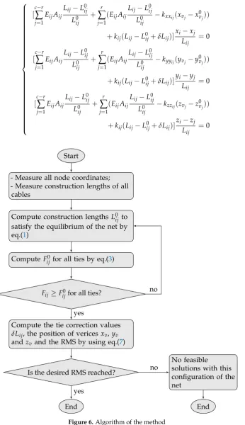
Start

- Measure all node coordinates; - Measure construction lengths of all

cables

Compute construction lengths L0_ij to satisfy the equilibrium of the net by eq.(1)

Compute F_ij0 for all ties by eq.(3)

Fij≥Fij0for all ties?

Compute the tie correction values δLij, the position of vericesxv,yv and zvand the RMS by using eq.(7)

Is the desired RMS reached?

No feasible solutions with this configuration of the net End End no yes no yes

Figure 6.Algorithm of the method

135

wherecis the total number of cables connected to thei-th node;ris the number of rods,xv,yv 136

andzvare the unknown coordinates of thej-th vertex andx0

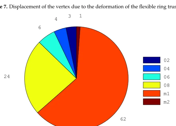
vertex itself. The stiffness of the truss support can be represented as a three-dimensional bushing, with 138

stiffnesseskxx_ij,kyy_ijandkzz_ij, connecting the rods to the vertex, as shown in Fig.7. The constrained 139

optimization (6) still applies to this flexible ring truss case and the overall algorithm is summarised in 140

the flowchart of Fig.6. 141

3. Results 142

In order to verify the validity of the proposed method, the case study of an asymmetric large 143

deployable reflector, designed by Thales Alenia Space [63], is described. Relevant parameters and 144

geometrical data are listed as follows: 145

• Focal length: 6 (m) 146

• Number of free nodes: 296 147

• Number of vertices: 14 148

• Number of total cables: 1044 149

• Cable section: 4 (mm)2 150

• Young modulus of cables: 8.3×1010(N/m)2 151

• Initial RMS error: 0.5872 (mm) 152

• Design value of the RMS faceting error: 0.21 (mm) 153

The value of spring constant in tie cables ranges from 2×103N/m to 68×103N/m with radial 154

step of 11×103N/m starting from the centre (central node) to the outer ring cables. The initial RMS 155

error on the front net was simulated by introducing an additional value to each node proportionally to 156

k

a b

ring truss support

rods

vertex

Figure 7.Displacement of the vertex due to the deformation of the flexible ring truss support

3 4 6

24

62 1

02 04 06 08 m1 m2

the length of the tie connected to it. By imposing the equilibrium in the system (1) we can determine the 157

construction lengths described in Section2. Nevertheless, from Fig.8it can be noted that the maximum 158

erroreL0obtained is about 1 (mm), representing only 1% of total cables; the largest percentage (86%) 159

showing an error between 0.6 (mm) and 1 (mm).

2000 3000 4000 5000 6000 7000 −2500

−2000 −1500 −1000 −500 0 500 1000 1500 2000 2500

0.5 0.55 0.6 0.65

Figure 9.Faceted RMS (mm) of the front tension truss in the initial configuration.

160

In Fig.9the local faceting error for the chosen initial configuration is shown. The local faceting 161

error is calculated considering the centroid of the triangular facets in which the surface can be 162

decomposed [64–67]. As it can be observed, the faceting error follows the shape of the asymmetric 163

reflector because the chosen error is proportional to the tie lengths. As a matter of fact, the central zone 164

is the one with the shortest cables and therefore with the lowest faceting error. On the contrary, the tie 165

lengths, and consequently the errors, grow moving from the centre to the outer perimeter of the net. 166

The optimization method described in the previous sections is first applied to the rigid ring truss 167

support. The Figure10shows the error of each free node of the front net with respect to the ideal 168

surface coupled with the stretching/shortening value necessary to reach the desired surface accuracy. 169

The reason why correction values are all positive is that the initial error is simulated by positioning all 170

nodes of the front net above the ideal surface, so there is the need to shorten the tie lengths to satisfy 171

the RMS design value. The bars are grouped by spring constant value. 172

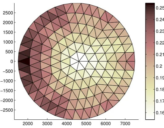
The corresponding faceting error is shown in Fig.11. As it can be observed the RMS of the faceting 173

error is lowered till the required value of 0.2036 (mm) furnished as specification. 174

Then, the same analysis has been performed for the flexible ring truss support. It can be noted that 175

in the Fig.12, the correction values are lower than the corresponding values with rigid truss support: 176

this is because the additional tensioning of ties further deforms the shape of the truss support resulting 177

in a closure of the support itself [68]. As a result, this causes a slight lowering of the front net thus 178

reducing the shortening action of tie lengths. Finally, the Fig.13shows the faceting error distribution 179

on the front net. Even in this case the final RMS faceting error reached 0.2045 (mm) representing 180

the design value of the RMS. Comparing the two Figs.11and13it can be observed that the faceting 181

error distribution is more uniform for the flexible ring truss support. This result can be explained 182

considering that the deformation of the truss support relaxes the front and rear tension truss systems 183

making the tension distribution more uniform. 184

Moreover, other simulations with different initial RMS errors revealed that, with the given design 185

−0.5 0 0.5

1 1.5

2 2.5

[mm]

Stretching/Shortening values Error

68 57 46 35 24 13 2

[N/mm]

Figure 10.Error and correction values (rigid case)

2000 3000 4000 5000 6000 7000

−2500 −2000 −1500 −1000 −500 0 500 1000 1500 2000 2500

0.17 0.18 0.19 0.2 0.21 0.22 0.23 0.24

Figure 11.Faceting error (mm) distribution on the front tension truss obtained for the rigid ring truss support

revision of design data is needed. This demonstrates the validity of the method only for small RMS 187

errors. 188

4. Conclusions 189

In this paper a method for the tie-system calibration of Large Deployable Reflectors (LDRs) is 190

provided. The LDRs are very sensitive to errors and usually require a careful experimental setup to 191

meet the design requirement of surface accuracy. Due to manufacturing errors, clearance, friction, not 192

perfect behaviour of materials the real configuration moves away from the design configuration and a 193

fine calibration is needed to improve the quality of the reflecting surface expressed in terms of closeness 194

to the ideal paraboloidal geometry. The proposed method follows two steps: the determination of the 195

−0.5 0 0.5

1 1.5

2 2.5

[N/mm]

[mm]

Stretching/Shortening values Error

68 57 46 35 24 13 2

Figure 12.Error and correction values (flexible case)

2000 3000 4000 5000 6000 7000

−2500 −2000 −1500 −1000 −500 0 500 1000 1500 2000 2500

0.16 0.17 0.18 0.19 0.2 0.21 0.22 0.23 0.24 0.25

Figure 13. Faceting error (mm) distribution on the front tension truss obtained for the flexible ring truss support

to meet RMS design requirements. For the first step a constrained optimization problem has been 197

proposed to find the cable construction lengths once all node coordinates have been measured. The 198

second step has been developed acting on the system of screw adjustable ties. A further constrained 199

optimization problem has been formulated to find the length corrections of each tie. Using the same 200

approach the cases of LDR with rigid and flexible tension truss have been studied. Finally, the method 201

has been applied to a LDR with asymmetrical ring truss designed by Thales Alenia Space. Considering 202

an initial RMS of 0.58 (mm) the results, not yet validated by experimental test, seemed comforting in 203

reaching the design RMS. The method convergency depends on the starting and desired RMS. Here, 204

the convergency has been insured up to the reasonable high initial RMS value of 1 (mm): beyond this 205

value the tie system is not able to reach the equilibrium and satisfy the constraints and a different 206

Author Contributions: This research paper was principally developed by the first and last author (A.C. and

208

P.D.M.). The other two authors (R.S. and R.R.) have dealt with the significant review activity.

209

Funding:“This research was funded by ESA grant number AO/1-7217/NL/CP - Innovative Scalable Large

210

Deployable Antenna Reflectors.”

211

Acknowledgments:This work has been partially financed by the University of Catania within the project “Piano

212

della Ricerca Dipartimentale 2016-2018” of the Department of Civil Engineering and Architecture.

213

Conflicts of Interest:“The authors declare no conflict of interest.”

214

Abbreviations 215

The following abbreviations are used in this manuscript:

216 217

MDPI Multidisciplinary Digital Publishing Institute DOAJ Directory of open access journals

TLA Three letter acronym

LD linear dichroism

218

References 219

1. Thomson, M. AstroMeshTM_{deployable reflectors for ku and ka band commercial satellites. 20th AIAA} 220

international communication satellite systems conference and exhibit, 2002, p. 2032.

221

2. Estler, W.T.; Edmundson, K.; Peggs, G.; Parker, D. Large-scale metrology–an update. CIRP

222

Annals-Manufacturing Technology2002,51, 587–609.

223

3. De Simone, M.C.; Guida, D. On the Development of a Low Cost Device for Retrofitting Tracked Vehicles

224

for Autonomous Navigation.Proceedings of the AIMETA2017.

225

4. Cuypers, W.; Van Gestel, N.; Voet, A.; Kruth, J.P.; Mingneau, J.; Bleys, P. Optical measurement techniques

226

for mobile and large-scale dimensional metrology. Optics and Lasers in Engineering2009,47, 292–300.

227

5. Dong, M.L.; Deng, W.Y.; Sun, Y.; Wang, Y. Photogrammetric Measurement of Deformation of Large

228

Deployable Mesh Microwave Antenna. Key Engineering Materials. Trans Tech Publ, 2008, Vol. 381, pp.

229

309–312.

230

6. Stegman, M.D.; Fedyk, M.; Kuehn, S. Solar thermal vacuum testing of deployable mesh reflector for model

231

correlation. Aerospace Conference, 2010 IEEE. IEEE, 2010, pp. 1–15.

232

7. Zhang, Y.; Li, Z.; Gao, J.; Hong, J.; Villecco, F.; Li, Y. A method for designing assembly tolerance networks

233

of mechanical assemblies. Mathematical Problems in Engineering2012,2012.

234

8. Villecco, F.; Pellegrino, A. Evaluation of uncertainties in the design process of complex mechanical systems.

235

Entropy2017,19, 475.

236

9. Villecco, F. On the evaluation of errors in the virtual design of mechanical systems. Machines2018,6, 36.

237

10. Cammarata, A.; Lacagnina, M.; Sinatra, R. Closed-form solutions for the inverse kinematics of the Agile

238

Eye with constraint errors on the revolute joint axes. Intelligent Robots and Systems (IROS), 2016 IEEE/RSJ

239

International Conference on. IEEE, 2016, pp. 317–322.

240

11. Cammarata, A. A novel method to determine position and orientation errors in clearance-affected

241

overconstrained mechanisms.Mechanism and Machine Theory2017,118, 247–264.

242

12. De Simone, M.; Guida, D. Dry friction influence on structure dynamics. Proceedings of the COMPDYN2015.

243

13. De Simone, M.C.; Guida, D. Modal Coupling in Presence of Dry Friction. Machines2018,6, 8.

244

14. Guida, D.; Pappalardo, C.M. Control design of an active suspension system for a quarter-car model with

245

hysteresis. JOURNAL OF VIBRATION ENGINEERING & TECHNOLOGIES2015,3, 277–299.

246

15. Pappalardo, C.M.; Guida, D. Adjoint-based optimization procedure for active vibration control of nonlinear

247

mechanical systems. Journal of Dynamic Systems, Measurement, and Control2017,139, 081010.

248

16. Pappalardo, C.M.; Guida, D. Control of nonlinear vibrations using the adjoint method.Meccanica2017,

249

52, 2503–2526.

250

17. Pappalardo, C.M.; Guida, D. A time-domain system identification numerical procedure for obtaining linear

251

dynamical models of multibody mechanical systems. Archive of Applied Mechanics2018,88, 1325–1347.

252

18. Pappalardo, C.M.; Guida, D. On the use of two-dimensional Euler parameters for the dynamic simulation

253

of planar rigid multibody systems. Archive of Applied Mechanics2017,87, 1647–1665.

19. Pappalardo, C.M.; Guida, D. System Identification Algorithm for Computing the Modal Parameters of

255

Linear Mechanical Systems. Machines2018,6, 12.

256

20. Pappalardo, C.M.; Guida, D. System Identification and Experimental Modal Analysis of a Frame Structure.

257

Engineering Letters2018,26.

258

21. Cavacece, M.; Pennestri, E.; Sinatra, R. Experiences in teaching multibody dynamics. Multibody System

259

Dynamics2005,13, 363–369.

260

22. Callegari, M.; Cammarata, A.; Gabrielli, A.; Sinatra, R. Kinematics and dynamics of a 3-CRU spherical

261

parallel robot. ASME 2007 International Design Engineering Technical Conferences and Computers and

262

Information in Engineering Conference. American Society of Mechanical Engineers, 2007, pp. 933–941.

263

23. Cammarata, A.; Angeles, J.; Sinatra, R. Kinetostatic and inertial conditioning of the McGill

264

Schönflies-motion generator. Advances in Mechanical Engineering2010,2, 186203.

265

24. Barbagallo, R.; Sequenzia, G.; Oliveri, S.; Cammarata, A. Dynamics of a high-performance motorcycle by

266

an advanced multibody/control co-simulation.Proceedings of the Institution of Mechanical Engineers, Part K:

267

Journal of Multi-body Dynamics2016,230, 207–221.

268

25. Barbagallo, R.; Sequenzia, G.; Cammarata, A.; Oliveri, S.; Fatuzzo, G. Redesign and multibody simulation

269

of a motorcycle rear suspension with eccentric mechanism. International Journal on Interactive Design and

270

Manufacturing (IJIDeM)2017, pp. 1–8.

271

26. De Simone, M.C.; Russo, S.; Rivera, Z.B.; Guida, D. Multibody model of a UAV in presence of wind fields.

272

Control, Artificial Intelligence, Robotics & Optimization (ICCAIRO), 2017 International Conference on.

273

IEEE, 2017, pp. 83–88.

274

27. Pappalardo, C.M.; Guida, D. Dynamic analysis of planar rigid multibody systems modeled using natural

275

absolute coordinates.Applied and Computational Mechanics2018,12.

276

28. Pappalardo, C.M.; Guida, D. On the Lagrange multipliers of the intrinsic constraint equations of rigid

277

multibody mechanical systems. Archive of Applied Mechanics2018,88, 419–451.

278

29. Pappalardo, C.M.; Guida, D. On the Computational Methods for Solving the Differential-Algebraic

279

Equations of Motion of Multibody Systems. Machines2018,6, 20.

280

30. Ghomshei, M.; Villecco, F.; Porkhial, S.; Pappalardo, M. Complexity in energy policy: A fuzzy logic

281

methodology. Fuzzy Systems and Knowledge Discovery, 2009. FSKD’09. Sixth International Conference

282

on. IEEE, 2009, Vol. 7, pp. 128–131.

283

31. Ghomshei, M.; Villecco, F. Energy metrics and Sustainability. International Conference on Computational

284

Science and Its Applications. Springer, 2009, pp. 693–698.

285

32. Sena, P.; Attianese, P.; Carbone, F.; Pellegrino, A.; Pinto, A.; Villecco, F. A fuzzy model to interpret data

286

of drive performances from patients with sleep deprivation. Computational and mathematical methods in

287

medicine2012,2012.

288

33. Sena, P.; d’Amore, M.; Pappalardo, M.; Pellegrino, A.; Fiorentino, A.; Villecco, F. Studying the influence of

289

cognitive load on driver’s performances by a Fuzzy analysis of Lane Keeping in a drive simulation. IFAC

290

Proceedings Volumes2013,46, 151–156.

291

34. Sena, P.; Attianese, P.; Pappalardo, M.; Villecco, F. FIDELITY: Fuzzy inferential diagnostic engine for on-line

292

support to physicians. 4th International Conference on Biomedical Engineering in Vietnam. Springer, 2013,

293

pp. 396–400.

294

35. Object Recognition by Using Neural Networks For Robotics Precision Agriculture Application, author=De

295

Simone, Marco Claudio and Guida, Domenico, journal=Engineering Letters, year=2018, publisher=under

296

review.

297

36. Salajegheh, E.; Salajegheh, J.; SEYEDPOUR, S.; Khatibinia, M. Optimal design of geometrically nonlinear

298

space trusses using an adaptive neuro-fuzzy inference system2009.

299

37. Finotto, V.C.; da Silva, W.R.; Valášek, M.; Štemberk, P. Hybrid fuzzy-genetic system for optimising

300

cabled-truss structures. Advances in Engineering Software2013,62, 85–96.

301

38. Pirrotta, S.; Sinatra, R.; Meschini, A. A novel simulation model for ring type ultrasonic motor.Meccanica

302

2007,42, 127–139.

303

39. De Simone, M.C.; Rivera, Z.B.; Guida, D. Obstacle Avoidance System for Unmanned Ground Vehicles by

304

Using Ultrasonic Sensors. Machines2018,6, 18.

305

40. Iannone, V.; De Simone, M.C. Modelling of a DC Gear Motor for Feed-Forward Control Law Design for

306

Unmanned Ground Vehicles.Actuators2018.

41. Zhai, Y.; Liu, L.; Lu, W.; Li, Y.; Yang, S.; Villecco, F. The application of disturbance observer to propulsion

308

control of sub-mini underwater robot. International Conference on Computational Science and Its

309

Applications. Springer, 2010, pp. 590–598.

310

42. De, S.; Rivera, Z.; Guida, D.; others. A new semi-active suspension system for racing vehicles. FME

311

Transactions2017,45, 578–584.

312

43. De Simone, M.C.; Guida, D. Identification and Control of a Unmanned Ground Vehicle By using Arduino.

313

UPB Sci. Bull. Ser. D2018,80, 141–154.

314

44. De, S.; Guida, D. Control design for an under-actuated UAV model.FME Transactions2018,46, 443–452.

315

45. Quatrano, A.; De, S.; Rivera, Z.; Guida, D. Development and implementation of a control system for a

316

retrofitted CNC machine by using Arduino.FME Transactions2017,45, 565–571.

317

46. Pellegrino, A.; Villecco, F. Design optimization of a natural gas substation with intensification of the energy

318

cycle. Mathematical Problems in Engineering2010,2010.

319

47. Formato, A.; Ianniello, D.; Villecco, F.; Lenza, T.L.L.; Guida, D. Design optimization of the plough working

320

surface by computerized mathematical model. Emirates Journal of Food and Agriculture2017, pp. 36–44.

321

48. Formato, A.; Guida, D.; Ianniello, D.; Villecco, F.; Lenza, T.; Pellegrino, A. Design of Delivery Valve for

322

Hydraulic Pumps. Machines2018,6, 44.

323

49. Muscat, M.; Cammarata, A.; Maddio, P.D.; Sinatra, R. Design and development of a towfish to monitor

324

marine pollution.Euro-Mediterranean Journal for Environmental Integration2018,3, 11.

325

50. Cammarata, A. Optimized design of a large-workspace 2-DOF parallel robot for solar tracking systems.

326

Mechanism and machine theory2015,83, 175–186.

327

51. Sequenzia, G.; Fatuzzo, G.; Oliveri, S.; Barbagallo, R. Interactive re-design of a novel variable geometry

328

bicycle saddle to prevent neurological pathologies. International Journal on Interactive Design and

329

Manufacturing (IJIDeM)2016,10, 165–172.

330

52. Barbagallo, R.; Sequenzia, G.; Cammarata, A.; Oliveri, S. An integrated approach to design an innovative

331

motorcycle rear suspension with eccentric mechanism. InAdvances on Mechanics, Design Engineering and

332

Manufacturing; Springer, 2017; pp. 609–619.

333

53. Cammarata, A.; Sinatra, R. On the elastostatics of spherical parallel machines with curved links. InRecent

334

Advances in Mechanism Design for Robotics; Springer, 2015; pp. 347–356.

335

54. Cammarata, A.; Caliò, I.; Greco, A.; Lacagnina, M.; Fichera, G.; others. Dynamic stiffness model of

336

spherical parallel robots. Journal of Sound and Vibration2016,384, 312–324.

337

55. Cammarata, A. Unified formulation for the stiffness analysis of spatial mechanisms. Mechanism and

338

Machine Theory2016,105, 272–284.

339

56. Cammarata, A.; Sinatra, R.; Maddio, P. A Two-Step Algorithm for the Dynamic Reduction of Flexible

340

Mechanisms. IFToMM Symposium on Mechanism Design for Robotics. Springer, 2018, pp. 25–32.

341

57. Cammarata, A.; Sequenzia, G.; Oliveri, S.M.; Fatuzzo, G. Modified chain algorithm to study planar

342

compliant mechanisms. International Journal on Interactive Design and Manufacturing (IJIDeM)2016,

343

10, 191–201.

344

58. Cammarata, A.; Lacagnina, M.; Sequenzia, G. Alternative elliptic integral solution to the beam deflection

345

equations for the design of compliant mechanisms. International Journal on Interactive Design and

346

Manufacturing (IJIDeM)2018, pp. 1–7.

347

59. De, S.M.C.; Rivera, Z.; Guida, D. Finite element analysis on squeal-noise in railway applications. FME

348

Transactions2018,46, 93–100.

349

60. Oliveri, S.; Sequenzia, G.; Calì, M. Flexible multibody model of desmodromic timing system.Mechanics

350

based design of structures and machines2009,37, 15–30.

351

61. Calì, M.; Oliveri, S.M.; Sequenzia, G. Geometric modeling and modal stress formulation for flexible

352

multi-body dynamic analysis of crankshaft. 25th Conference and Exposition on Structural Dynamics, 2007,

353

pp. 1–9.

354

62. Pappalardo, C.M. A natural absolute coordinate formulation for the kinematic and dynamic analysis of

355

rigid multibody systems. Nonlinear Dynamics2015,81, 1841–1869.

356

63. Maddio, P.; Meschini, A.; Sinatra, R.; Cammarata, A. An optimized form-finding method of an asymmetric

357

large deployable reflector. Engineering Structures2019,181, 27–34.

358

64. Agrawal, P.; Anderson, M.; Card, M. Preliminary design of large reflectors with flat facets.IEEE transactions

359

on antennas and propagation1981,29, 688–694.

65. Li, P.; Liu, C.; Tian, Q.; Hu, H.; Song, Y. Dynamics of a deployable mesh reflector of satellite antenna:

361

form-finding and modal analysis. Journal of Computational and Nonlinear Dynamics2016,11, 041017.

362

66. Yuan, S.; Yang, B.; Fang, H. Improvement of Surface Accuracy for Large Deployable Mesh Reflectors.

363

AIAA/AAS Astrodynamics Specialist Conference, 2016, p. 5571.

364

67. Morterolle, S.; Maurin, B.; Quirant, J.; Dupuy, C. Numerical form-finding of geotensoid tension truss for

365

mesh reflector.Acta Astronautica2012,76, 154–163.

366

68. Liu, W.; Li, D.X.; Yu, X.Z.; Jiang, J.P. Exact mesh shape design of large cable-network antenna reflectors

367

with flexible ring truss supports. Acta Mechanica Sinica2014,30, 198–205.