Efficiently Processing Complex-Valued Data in Homomorphic Encryption

Efficiently Processing Complex-Valued Data in

Homomorphic Encryption

Carl Bootland1_{, Wouter Castryck}1,2_{, Ilia Iliashenko}1_{, and Frederik} Vercauteren1

1_{imec-COSIC, Dept. Electrical Engineering, KU Leuven}

[email protected]

2

Department of Mathematics, KU Leuven

Abstract. We introduce a new homomorphic encryption scheme that is natively capable of computing with complex numbers. This is done by generalizing recent work of Chen, Laine, Player and Xia, who modified the Fan–Vercauteren scheme by replacing the integral plaintext modulus t by a linear polynomial X −b. Our generalization studies plaintext moduli of the formXm_{+b. Our construction significantly reduces the}

noise growth in comparison to the original FV scheme, so much deeper arithmetic circuits can be homomorphically executed.

1

Introduction

The goal of homomorphic encryption is to allow for arbitrary arithmetic opera-tions on encrypted data, such that the decrypted result equals the outcome of the same calculation carried out in the clear. Since the publication of Gentry’s seminal Ph.D. work [15], this research area has evolved rapidly and is on the verge of reaching a first degree of maturity, as was recently demonstrated e.g. by practical implementations of privacy-enhanced electricity load forecasting [3, 2], digital image processing [1, 10], and medical data management [12, 18, 7]. Most of the current focus lies on somewhat homomorphic encryption (SHE), where the schemes are capable of homomorphically evaluating an arithmetic circuit having a certain predetermined computational depth. The leading proposals for realizing this goal are the Brakerski-Gentry-Vaikunthanathan (BGV) scheme [4] and the Fan-Vercauteren (FV) scheme [13].

In actual applications, the input to the homomorphic evaluation of an arith-metic circuitC needs to be preprocessed in two steps. The first step is encoding, where one’s task is to represent the actual ‘real world data’ as elements of the plaintext space of the envisaged SHE scheme. This plaintext space is a certain commutative ring, and the encoding should be such that real world arithmetic

agrees with the corresponding ring operations, up to the anticipated computa-tional depth.

In the original descriptions of BGV and FV, the plaintext space is a ring of the form Rt = Z[X]/(t, f(X)) where t ≥ 2 is an integer and f(X) ∈ Z[X]

is a monic irreducible polynomial. Throughout this paper we will stick to the common choice of 2-power cyclotomics f(X) =Xn_{+ 1, where n= 2}k _{for some}

integer k≥1. Encoding numerical input is typically done by taking an integer-digit expansion with respect to some base b, then replacing b byX and finally reducing the digits modulo t. Decoding then amounts to lifting the coefficients back to_Z, for instance by choosing representatives in (−t/2, t/2], and evaluating the result atX=b. Thanks to the relationX−1_{≡ −X}n−1_{it is possible to allow} the expansions to have a fractional part. In this case the decoding step must be preceded by replacing the monomials Xi _{of degree i > B by−X}i−n_{, for some}

appropriate point of separation B. All these parameters need to be chosen in such a way that the evaluation of C on the encoded data decodes to the right outcome. At the same time one wantstto be as small as possible, because its size highly affects the efficiency of the resulting SHE computation. Selecting optimal parameters is a tedious application-dependent balancing act to which a large amount of recent literature has been devoted, see e.g. [20, 12, 8, 6, 18, 11, 2].

Because in practicenis of size at least 1024, the plaintext spacesRtcan a pri-ori host an enormous range of data, even for very small values oft. Unfortunately this is hindered by their structure, which is not a great match with numerical input data types like integers, rationals or floats. For example, ift= 2 then it is not even possible to add a non-zero element to itself without incorrect decoding. Because of such phenomena, values of t are required that typically consist of dozens of decimal digits, badly affecting the efficiency. An idea to remedy this situation has been around for a while [17, 4, 14] and uses a polynomial plaintext modulus, rather than just an integer. Recently the first detailed instantiation of this idea was given by Chen, Laine, Player and Xia [6], who adapted the FV scheme to plaintext modulit=X−bfor someb∈Z≥2. In this case the plaintext space becomes Rt = Z[X]/(X−b, Xn+ 1) = Z[X]/(X −b, bn+ 1) ∼=Zbn₊₁,

whose structure is amuch better match with the common numerical input data types. This allows for much smaller plaintext moduli (norm-wise), with benefi-cial consequences for the efficiency, or for the depth of the circuitsCthat can be handled [6, Section 7.2].

This paper further explores the paradigm that the structure of the plaintext space Rt should match the input data type as closely as possible. Concretely,

Representing complex numbers. One naive way to encode a complex num-berzwould be to view it as a pair of real numbers, for instance using Cartesian or polar coordinates. These can be fed separately to the SHE scheme, which is now used to evaluate two circuits. A more direct way is to use a complex base

b. For instance, one could takeb=eπi/n_{, as was done by Cheon, Kim, Kim and}

Song [8], albeit in a somewhat different context. This choice has the additional feature thatf(b) = 0, so that wrapping around modulof(X) =Xn_{+ 1 does not}

lead to incorrect decoding. However, finding an integer-digit base b expansion with small norm which approximatesz sufficiently well is ann-dimensional lat-tice problem, which is practically infeasible. To get around this Costache, Smart and Vivek [10] instead useb=ζ:=eπi/mfor some divisorm|n, which is small enough for finding short base ζ approximations, while preserving the feature that wrapping around modulof(X) is unharmful. But in their approach, a huge portion of plaintext space is leftunused. Indeed, the encoding map is

Z[ζ]→Rt:z= m−1

X

i=0

zibi7→ m−1

X

i=0

ziYi,

whereY =Xn/m,t≥2 is an integral plaintext modulus andziis the reduction of zi mod t, so that all plaintext computations are carried out in the subring

Z[Y]/(t, Ym+ 1), which is of index tn−m in Rt. Our proposal is to resort to

a plaintext modulus of the form t = Xm_{+b for some small integer b, with}

|b| ≥2. In this case, for m < n, we have RXm_+b =_Z[X]/(Xm+b, Xn+ 1) =

Z[X]/(bn/m+ 1, Xm+b). An additional assumption (which is discussed in more

detail in the next section), is that

there exists anα∈Zbn/m₊₁ such thatb=αm, (1)

wherebdenotes the reduction ofbmodulobn/m+ 1. Throughout we fix such an

αand let β be its multiplicative inverse, which necessarily exists. This implies that ( ¯βX)m+ 1 = 0, therefore we have a well-defined ring homomorphism

Z[ζ]→RXm_+b :

m−1 X

i=0

ziζi7→ m−1

X

i=0

ziβ i

Xi (2)

which is surjective with kernel (bn/m+ 1). In other words, while Costache, Smart and Vivek restrict their computations to an injective copy ofZ[ζ]/(t) insideRt,

we can viewRXm_+b as an isomorphic copy of _Z[ζ]/(bn/m+ 1). Essentially, our

approach transfers the unused part of the plaintext space coming from the large dimensionninto a larger integral modulus, reflected in the exponentn/m.

cyclotomic rationals or complex floats, either by resorting to LLL as in [10] or by using Chen et al.’s fractional encoder from [6]. In Section 4 we discuss how to adapt the FV scheme so that it can cope with plaintext spaces of the form

RXm+b. Finally, in Section 6 we discuss the performance of this adaptation in

comparison with previous approaches. In short we can reach a depth at least 5 times that of the best approach which directly encrypts encodings of complex numbers [10]. We can also reach very similar depths to the state of the art where one encrypts the real and imaginary parts separately [6]. However, since we natively encrypt complex numbers our ciphertexts are two times smaller and hence our approach is more efficient by roughly a factor two in time and three in space.

2

Encoding and decoding elements of

_Z

[

ζ

]

Encoding Encoding an element of Z[ζ] happens in two steps. The first step

applies the map (2) yielding a polynomial of degree less thanmwhich typically has very large coefficients. The second step is comparable to the hat encoder of Chen et al. [6] and switches to another representant by spreading this polynomial across the range 1, X, . . . , Xn−1 _{while making the coefficients a lot smaller. The} result will then be lifted to R =_Z[X]/(Xn_{+ 1) and fed to our adaptation of}

the FV scheme, where the smaller coefficients are important to keep the noise growth bounded.

Here is how this second step is carried out in practice: we think of the coef-ficientsziβ

i

as being represented by integers between−bbn/m_/2canddbn/m_/2e.

We then expand these integers to basebusing digitsai,j from the range−bb/2c,

. . . ,bb/2cto find

ziβ i

=ai,n/m−1b

n/m−1

+. . .+ai,1b+ai,0.

There is a minor caveat here, namely if b is odd then there are more integers modulo bn/m+ 1 than there are balanced b-ary expansions of length at most

n/m. This is easily resolved by allowing the last digit to be one larger. For even

bthe situation is opposite: sinceziβ i

is represented by an integer of size at most

bn/m_{/2 = b/2·b}n/m−1 _{we have a surplus of base-b expansions. Here it makes} sense to choose an expansion with the shortest Hamming weight (e.g., ifb = 2 then we simply pick the non-adjacent form). We denote the maximal number of non-zero coefficients that can appear in a fresh encoding byNb.

Given such base-bexpansions of the coefficients, we replace each occurrence of

b by−Xm_{and then substitute the results in the image of (2). We end up with}

an expansion Pn−1

i=0 ciX

i _{where the ci are represented by integers of absolute}

value at most bb/2c, or in fact b(b+ 1)/2cif we take into account the caveat.

Decoding In order to decode a given expansion Pn−1

i=0 ciX

i _{we walk through}

the expansion moduloXm_{+b, in order to end up with}

m−1 X

i=0

c0_iXi ∈_Z[X]/(bn/m+ 1, Xm+b).

This can be rewritten as Pm−1

i=0 c 0

iα

i_βi_Xi _{so we decode as} Pm−1

i=0 ziζ

i _∈

Z[ζ]

whereziis a representant ofc0_iαitaken from the range−bbn/m_{/2c, . . . ,db}n/m_/2e.

On the assumption (1) Usuallynandm are determined by security consid-erations and the concrete application. To apply our encoding method we want to find a small value ofb for which condition (1) is met. This is easiest ifn/m

is small or m is small. If no satisfactory value of b can be found then one can try to enlargemand view_Z[ζ] as a subring of a higher degree cyclotomic ring. Below we give two lemmas constraining the possible choices for b givenm and

n; still assuming we are working with 2-power cyclotomicf.

One choice forb which is always possible is 2m/2_{, since definingαas}

α= 2n/82n/4−1, (3)

then it easy to verify thatα2_{≡2 mod 2}n/2_{+ 1 and hence}

αm≡2m/2mod 2m2 mn _{+ 1.}

If m is small then this results in a reasonably slow coefficient growth. On the other hand if m is large compared to n then the modulus bn/m_{+ 1 is smaller}

and it is apparently easier to have condition (1) satisfied, as is confirmed by experiment.

Lemma 1. Let n > m >1. A necessary condition for (1)is that for every odd primep|bn/m_{+ 1we have 2n|p−1.}

Proof. First we show thatb has multiplicative order 2n/min_Zbn/m₊₁. Clearly

we havebn/m≡ −1 modbn/m+ 1 so thatb2n/m≡1 modbn/m+ 1. This shows that the order ofbdivides 2n/mso is a power of 2 and hence it is equal to 2n/m. Since 2 | n/m and x2 _{≡ 1 mod 4 for any odd xwe have that if b is odd}

bn/m_{+ 1≡2 mod 4 while ifb is evenb}n/m_{+ 1 is odd. Thus that we can write}

bn/m+ 1 = 2ρpe1

1 . . . p

ej

j

where thepi, 1≤i≤j are distinct odd primes andρ=bmod 2.

Now we can see via the Chinese Remainder Theorem that there exists anα

such that αm_{≡b modb}n/m_{+ 1 if and only if there existα}

i such that αim≡b

modpei

i for every i. Further we must have bn/m ≡ −1 modp ei

i so that b has

order 2n/m modulopei

i . This implies αi has orderm·2n/m= 2n modulop ei

i

and since (_Z/pei

i Z)× is cyclic of orderp ei−1

i (pi−1) we see that 2n|(pi−1) by

Lemma 2. Let g be an element of order n in _Z×_4n and let t be an element of order 2 not in hgi so that _Z4×_n =hti × hgi. If condition (1) is satisfied for odd

b > 1 and m >1 then bmod 4n is an element of the subgroup hti × hgm_{i. In}

particular this implies that b≡ ±1 mod 4m.

In fact, one may always takeg= 3 and t=−1 in the above lemma.

Proof. Using Lemma 1 and the notation from its proof we can write eachpi as 2nci+ 1 for some natural numberci. This implies that

bn/m+ 1 = 2

j

Y

i=1

(2nci+ 1)ei _{≡2 mod 4n}

and hence bn/m ≡ 1 mod 4n. Therefore the order of b as an element of Z×4n

dividesn/m.

Now we haveZ×4n=hti × hgiso that forbmod 4nto have an order dividing n/m it must be an element of the subgroup hti × hgmi. This is because this subgroup certainly only contains elements whose order divides n/m. Further,

Z×4n has exactly 2n/msuch elements but this is the size of the subgroup so the

subgroup is exactly all such elements.

For the final part we note, as stated after the lemma, thatg= 3 andt=−1 can be taken and that 3m_{≡1 mod 4mwhich gives the desired result. We remark}

that for anyb≡ ±1 mod 4mit is always the case thatbn/m_{≡1 mod 4nso from}

this condition we cannot determine anything more aboutb modulo 4m but the condition given modulo 4nis stronger.

Lemma 3. Supposeb,nand msatisfy (1), then so does−b, n, m.

Proof. Since (−b)n/m+ 1 =bn/m+ 1 whennis a power of two and m < n, we must show that −1 has an mth root modulo bn/m_{+ 1; we show thatα}n/m _is

such anmth root. We have (αn/m₎m_{= (α}m₎n/m_≡bn/m_{≡ −1 modb}n/m_{+ 1 as}

required. Hence we see that (αn/m+1₎m_=αn_αm_{=−1·bas required.}

We note that the above proof only required n/mto be even and not equal to a power of two so applies somewhat more generally.

Our method is particularly friendly towards Gaussian integers. Indeed ifm= 2 then one can always takeb= 2, as we have seen thatα2= 2 whereαis as in (3). The map (2) then defines an isomorphism betweenRX2₊₂ and _Z[i]/(2n/2+ 1).

If this ring is not large enough to ensure correct decoding, then one can move to slightly larger values of b. The next choice which always works isb = 4, where one can simply takeα= 2. Here the ring becomesZ[i]/(2n+ 1).

3

Encoding complex-valued input data

by suitable cyclotomic rationals and then proceed as in Section 2. We have many choices for such approximations including the choice of m which defines which root of unity we are working with. We also have the choice between using integer or rational coefficients for the approximation. Perhaps the most obvious and straightforward approach is to consider our complex number z written in terms of its real and imaginary parts, say z = x+yi for some real numbers

x and y. We can then approximate x and y by rationals depending on how much precision we require. This leads us to considering the case m= 2 and the question then arises of how to encode fractional coefficients.

3.1 Fractional encoding

Here we consider how to encode a rational number into the space Z/pZ for

some integer p, so that it can then be expanded using the technique in Section 2. This problem was considered by Chen, Laine, Player and Xia in [6, Section 6]. Their approach is to define a finite subset P of Q along with an encoding

mapEnc:P →Z/pZand a decoding mapDec:Enc(P)→ P. The maps should

satisfy, firstly, correctness: Dec(Enc(x/y)) =x/y forx/y ∈ P and secondly,Enc should be both additively and multiplicatively homomorphic so long as it still encodes an element ofP. The natural choice for the mapEncisEnc(x/y) =xy−1 modpwhere the inverse ofyis computed modulop. Care thus needs to be taken to ensure thaty has such an inverse, which is ensured with a careful choice of P.

In our setting the coefficient modulus pis of the form bn/2+ 1, thus if one wants roughly the same precision for the integer and fractional parts one can take for an odd baseb

P=

c+ d

bn/4 : c, d∈

−b

n/4₋₁

2 ,

bn/4−1 2

∩Z

;

while for evenbone can choose

P=

c+ d

bn/4−δ :|c| ≤

(bn/4+δ−1_−1)b 2(b−1) ;|d| ≤

(bn/4−δ_−1)b

2(b−1) ;c, d∈Z

,

where δ ∈ {0,1} depending on whether you want one more base-b digit in the fractional (δ= 0) or integer (δ= 1) part.

We note that the fractional encoder need not require m to be 2. However in this case there appears to be no straightforward way to find a good rational approximation with small numerators and denominators except when the de-nominators are all equal, in this case if this denominator is r then we simply require an approximation ofrz inZ[ζ] subject to some constraint on the

coeffi-cients. However, the problem of finding such an approximation to our complex number itself, rather than a scaling, is interesting in its own right as it avoids the need for encoding fractional values and tracking the denominator inherently present in such encodings.

3.2 Integer coefficient approximation

The task of finding a cyclotomic integer closely approximating an arbitrary com-plex number was considered by Costache, Smart and Vivek in [10]. Here the idea is to solve an instance of the closest vector problem (CVP) in the (scaled) lattice

Z[ζ], where the power basis is scaled and split into real and complex part, which

are approximated by integers. In detail: we choose a scaling constantC >0, and define the constants ai and bi for i = 0, . . . , m−1, whereai = d<(Cζi_{)c and} bi=d=(Cζi_{)c. The lattice we then consider is given by themrows of the matrix}



 

1 0 a0 b0 . ._. .._. .._. 0 1am−1bm−1



 .

The target vector in our CVP instance will then be the appropriately scaled real and complex parts of the complex numberzwe wish to approximate. Concretely, this vector is (0, . . . ,0,d<(Cz)c,d=(Cz)c).

If (z0, . . . , zm−1, A, B) is a solution to the CVP instance then we must have

d<(Cz)c ≈A=

m−1 X

i=0

ziai≈ < C m−1

X

i=0

ziζi

!

and similarly for the imaginary part. We therefore see thatPm−1

i=0 ziζ

i _{is a good}

approximation toz. Further,Cgives some control over the quality of the approx-imation, larger C gives a finer-grained lattice but also increases the size of the last two coefficients of the basis vectors which may lead to a larger distance be-tween the target vector and the closest lattice point, which in turn makes solving the CVP instance harder and negatively affects the quality of our approximation ofCz.

In [10] the authors solve this CVP instance using the embedding technique. Namely they attempt to solve the shortest vector problem in the lattice spanned by the rows of



   

1 0 a0 b0 0

. ._. .._. .._. .._. 0 1 am−1 bm−1 0 0· · · 0d<(Cz)c d=(Cz)cT



for some non-zero constantT. With suitable parameter choices, performing LLL reduction on this lattice will return a basis of short vectors for this lattice, among which at least one has±Tin the final coordinate. The remaining coefficients then give plus or minus the target vector minus a close vector.

One issue with the embedding technique is that each new instance of the CVP problem requires performing lattice reduction which for largem is rather time-consuming. In typical applications we want to approximate many different complex numbers, using the same Cso only the target vector changes. A more efficient approach therefore is to perform lattice reduction on the CVP lattice itself and since this is independent of the target vector it needs only to be done once so we can spend significantly more time in this step to find a good basis of this lattice. We can then apply a technique such as Babai’s nearest plane algorithm, or Babai’s rounding algorithm, with this reduced basis to find an approximate closest vector.

4

Adapting the Fan-Vercauteren SHE scheme

In this section we construct a variant of the FV scheme [13] with plaintext modulus Xm_{+b following the blueprint given in [6]. We prove correctness of}

this scheme and analyze the noise growth induced by homomorphic arithmetic operations.

4.1 Basic scheme

Writing R = _Z[X]/(Xn_{+ 1), the ciphertext space is defined by R}

q = R/(q)

for some positive integerq, while the plaintext space is RXm_+b=R/(Xm+b).

We will assume thatbq. Recall that in the original FV scheme the plaintext space isR/(t) for some positive integertq. We define the scaling parameter

∆b as

∆b=

_q

Xm_+b mod (X n_{+ 1)}

=

   −

q bn/m_{+ 1}

n/m

X

i=1

(−b)i−1Xn−im



  

.

Obviously,∆bis the analogue of the scalar∆=bq/tcin the original FV scheme. Other parameters are the error distribution χe =D(σ2_{) on R (coefficient-wise} with respect to the power basis, with standard deviationσ) and the key distribu-tionχk =U3 which uniformly generates elements of Rwith ternary coefficients (with respect to the power basis). We also define the decomposition basewand denote`=blogwqc.

The new encryption scheme ComFV is then defined in the same way as FV wheret and∆are replaced byXm+band ∆b, respectively.

• ComFV.KeyGen( ): Lets←χk ande, e0, . . . e` ←χe. Uniformly sample

ran-doma, a0, . . . , a`∈Rq and compute bi=

−(ais+ei) +wis2

q. Output the

• ComFV.Encrypt(pk,msg): Sampleu←χkande0, e1←χe. Setp0=pk[0] and

p1 =pk[1], and compute c0 = [∆b·msg+p0u+e0]q and c1 = [p1u+e1]q.

Outputct= (c0, c1).

• ComFV.Decrypt(sk,ct): Returnmsg0=jXm_q+b[c0+c1s]q

m

mod (Xm+b).

The security of this scheme is based on the same argument as of the orig-inal FV scheme. In particular, it is hard to distinguish the public key pk and ciphertext pairs from uniform tuples according to the decision version of the Ring-LWE problem [19]. The evaluation key evkdoes not leak any information about the secret key as long as a circular security assumption holds [13].

For an elementa∈ K := _Q[x]/(f(x)) the canonical (infinity) norm of a is defined as

kakcan_∞ = a(ζ), a(ζ3), . . . , a(ζ2n−1)

∞.

In Appendix A we state some properties of the canonical norm which will be used throughout this section. To verify correctness we use the notion of invariant noise introduced in [6]. Theinvariant noise of a ciphertextct= (c0, c1) encrypting a plaintext msg∈RXm_+b is an element v∈K with the smallest canonical norm

such that

Xm_+b

q ·[c0+c1s]q =msg+v+g(X

m_{+b) (4)}

for some g ∈ R. Then decryption works correctly when kvkcan_∞ < 1/2 that is supported by the following theorem.

Theorem 1 (Decryption noise). Let ct be an encryption of the plaintext element msg ∈ RXm_+b such that its invariant noise v satisfies kvkcan

∞ < 1/2. ThenComFV.Decrypt(sk,ct) =msg.

Proof. Computing ComFV.Decrypt(sk,ct), we have using the definition of the invariant noise

msg0=

_Xm_+b

q [ct[0] +ct[1]·s]q

mod (Xm+b)

=bmsg+v+g(Xm+b)emod (Xm+b) =msg+bve

for some g ∈ R and since kvk_∞ ≤ kvkcan_∞ < 1/2 we have bve = 0. Thus

msg0 =msg.

To show that v is small enough, we need an upper bound on the initial invariant noise size depending on the scheme parameters. For this purpose, we use the heuristic approach of Gentry et al. [16]. This approach relies on the average distributional analysis, which estimates the expected size of the invariant noise in the canonical embedding norm.

at most one coefficient reaching this bound. Hence,kmsgkcan_∞ ≤Nb(b+1)/2. Now,

we have all the ingredients to define the scheme parameters supporting correct decryption.

Fresh noise heuristic. Let ct=ComFV.Encrypt(pk,msg) be a fresh ciphertext. Setc0=ct[0],c1=ct[1], andp0=pk[0], p1=pk[1]. We have, working modulo (Xm_{+b), that}

Xm_+b

q ·[c0+c1s]q =

Xm_+b

q ·(∆b·msg+p0u+e0+p1us+e1s) (5)

For some polynomialg∈K withkgk_∞≤1/2,

∆b(Xm+b)

q =

_q

Xm_+b +g

·X

m_+b

q = 1 +

g(Xm_+b)

q .

Thus we can takeρ=g(Xm+b)∈K and

kρkcan_∞ =kg(Xm+b)kcan_∞ ≤(b+ 1)√3n, (6)

where the last inequality holds with very high probability due tog(X)← Urnd; see Appendix A. Now, we can expand (5) as follows

Xm_+b

q ·[c0+c1s]q=msg·

1 + ρ

q

+X

m_+b

q ·(p0u+e0+p1us+e1s)

=msg+ρ

q·msg+

Xm+b

q ·((−as−e)u+aus+e1s)

=msg+ρ

q·msg+

Xm_+b

q ·(−eu+e1+e2s)

Here, the noisy term isv= (ρ·msg+ (Xm_{+b)·(−eu+e}

1+e2s))/q. Given (6) and the canonical norm analysis in Appendix A, it follows that

kvkcan_∞ ≤1

q ·

(b+ 1)Nb√3n· b+ 1

2 + 6(b+ 1) √

npσ2_{(4n/3 + 1)}

=b+ 1

q ·

√ 3n

2 ·(b+ 1)Nb+ 2σn r

12 +9

n

!

.

4.2 Homomorphic operations

In this section we show how homomorphic addition and multiplication are per-formed in the new scheme. We prove correctness of these operations and estimate the invariant noise growth. Throughout this section,Ct(msg, v) denotes a cipher-text encrypting messagemsg∈RXm+b with invariant noisev.

Addition is the coordinate-wise sum of corresponding ciphertext components:

It follows immediately from (4) that the invariant noise grows additively as in the lemma below.

Lemma 4 (Addition noise). Given two ciphertexts ct1 = Ct(msg1, v1) and ct1=Ct(msg2, v2), the functionComFV.Add(ct1,ct2)returns a ciphertextctAdd=

Ct(msg₁+msg₂, vAdd)with kvAddk

can ∞ ≤ kv1k

can ∞ +kv2k

can ∞ .

Multiplication consists of two steps. The first one, denotedComFV.BMul, re-turns the coefficients of the ciphertext product when expressed as of a polynomial in s, namely of (ct0[0] +ct0[1]s)(ct1[0] +ct1[1]s). The second step then maps the degree two term back to degree one using the relinearization technique.

• ComFV.BMul(ct0,ct1): Computec0= hj

Xm_+b

q ·ct0[0]·ct1[0]

mi

q

,

c1= hj

Xm_+b

q ·(ct0[0]·ct1[1] +ct0[1]·ct1[0])

mi

q

andc2= hj

Xm+b

q ·ct0[1]·ct1[1]

mi

q

.

ReturnctBMul= (c0, c1, c2).

• ComFV.Relin(ctBMul,evk): WritingctBMul = (c0, c1, c2), expand c2 in base w, namelyc2=P

`

i=0c2,iwi withc2,i∈Rw. Compute

c0₀= "

c0+

`

X

i=0

evk[i][0]·c2,i

#

q

, c0₁= "

c1+

`

X

i=0

evk[i][1]·c2,i

#

q

and outputcRelin= (c00, c01).

• ComFV.Mul(ct0,ct1,evk): ReturncMul=ComFV.Relin(ComFV.BMul(ct0,ct1),evk).

To estimate the noise growth of multiplication, we analyze each step above separately. First, we provide a heuristic upper bound on the noise introduced by ComFV.BMul.

Noise heuristic afterComFV.BMul. Given two ciphertextsct1=Ct(msg1, v1) and ct1=Ct(msg2, v2), the functionComFV.BMul(ct1,ct2) returns a triplectBMul=

(c0, c1, c2) According to the description of ComFV.BMul, every component ci of

ctBMul contains a rounding errorri, krik∞≤1/2. Thus, decryptingctBMul leads

to

Xm_+b

q ·

c0+c1s+c2s2_q=

_Xm_+b q

2

·ct1(s)·ct2(s) +r+g(Xm+b),

where r= (Xm+b)(r0+r1s+r2s2)/q andg ∈R. According to Appendix A, the variance ofr0+r1s+r2s2

can

∞ is equal ton/12 +n

2_{/18 +n}3_{/27. It follows} that

krkcan_∞ ≤ b+ 1

q 6

p

n/12 +n2_{/18 +n}3_/27

= b+ 1

q

p

Since (Xm_+b)·

cti(s)/q=msgi+vi+gi(Xm+b) for somegi∈R, expanding

the previous expression results in

Xm+b

q ·

c0+c1s+c2s2_q =msg1·msg2+v2(msg1+g1(Xm+b))

+v1(msg2+g2(Xm+b)) +v1v2+r

+ (msg₁·g2+msg2·g1+g)(Xm+b) +g1g2(Xm+b)2

=msg₁·msg₂+vBMul+h(Xm+b).

Notice thatcti[0] andcti[1] should be indistinguishable from samples generated

by Uq according to the decision Ring-LWE problem. The variance of cti[0] +

cti[1]·sis thusq2n/12 +q2n2/18. Hence, it follows

kmsg_i+gi(Xm+b)kcan_∞ =

Xm_+b

q ·cti(s)−vi

can

∞

≤ b+ 1

q ·q

p

3n+ 2n2_+kv

ik

can ∞

= (b+ 1)p3n+ 2n2_+kv

ik

can ∞ .

Hence, the noisy termvBMul satisfies

kvBMulk

can ∞ ≤ kv2k

can ∞ ·

(b+ 1)p3n+ 2n2_+kv 1k

can ∞

+kv1kcan_∞ ·(b+ 1)p3n+ 2n2_+kv2kcan ∞

+kv1k can ∞ · kv2k

can ∞ +

b+ 1

q

p

3n+ 2n2_{+ 4n}3_/3.

Finally, we obtain

kvBMulk

can

∞ ≤(b+ 1) p

3n+ 2n2_(kv1kcan ∞ +kv2k

can

∞ ) + 3kv1k can ∞ · kv2k

can

∞ (7)

+b+ 1

q

p

3n+ 2n2_{+ 4n}3_/3

with very high probability.

Next, we provide a heuristic upper bound on the noise introduced after re-linearization.

relinearization

Xm_+b

q ·[ctRelin(s)]q=

Xm_+b q ·[c

0

0+c01s]q

= X

m_+b

q · c0+c1s+c2,i `

X

i=0

evk[i][0] +evk[i][1]·s

!

+g(Xm+b)

= X

m_+b

q · c0+c1s− `

X

i=0

eic2,i+s2 `

X

i=0

wic2,i

!

+

`

X

i=0

gic2,i+g

!

(Xm+b).

Recall that by definition P

iw i_c

2,i=c2. Thus, replacingPigic2,i+g by ˜g, we

obtain for someh∈R

Xm_+b

q ·[ctRelin(s)]q =

Xm_+b

q · c0+c1s+c2s

2₋

`

X

i=0

eic2,i

!

+ ˜g(Xm+b)

=msg+v−X

m_+b

q ·

`

X

i=0

eic2,i+ (˜g+h)(Xm+b)

As a result, vRelin = v− X

m_+b

q ·

P`

i=0eic2,i. Given that c2,i’s look uniformly

random inRw, the variance of P`

i=0eic2,iis equal to (`+ 1)(wσn)2/12. Hence,

we obtain

kvRelink

can ∞ ≤ kvk

can ∞ +

b+ 1

q ·

`

X

i=0

keic2,ik

can ∞

≤ kvkcan_∞ +b+ 1

q ·6σnw

r

`+ 1 12 .

As a result, the relinearization noise satisfies

kv_Relinkcan_∞ ≤ kvkcan_∞ +b+ 1

q ·σnw

p

3(`+ 1) (8)

with very high probability.

Noise heuristic after ComFV.Mul. Combining the two previous heuristics (7) and (8), we deduce the total noise growth after homomorphic multiplication. Given two ciphertextsct1=Ct(msg1, v1) andct1=Ct(msg2, v2), the function ComFV.Mul(ct1,ct2,evk) outputs a ciphertextctMul=Ct(msg1·msg2, vMul) with

kvMulk

can ∞ (b+ 1)

p

3n+ 2n2_(kv1kcan ∞ +kv2k

can

∞ ) + 3kv1k can ∞ · kv2k

can ∞

+b+ 1

q

p

3n+ 2n2_{+ 4n}3_{/3 +}b+ 1

q ·σnw

p

with very high probability. We note that the dominating term here is the first term and not the term containing the product of the canonical norms of the multiplicands since the canonical norms are smaller than 1/2 when the ciphertext can be decrypted correctly.

5

Application to Image Processing

In this section we apply theComFVscheme to the image processing use case [10]. For this application, as with any other, we need to take into account two con-straints regarding computation correctness. Firstly, the coefficients of encrypted encodings can increase in absolute value after arithmetic operations and reach some bound, say, B. To decode these resulting encodings, B must be smaller than (bn/m+ 1)/2 as described in Section 3. Secondly, the invariant noise of encryptions grows as well according to the heuristic estimates of Section 4. To decrypt the resulting output, this noise should be smaller than 1/2 as shown in Theorem 1.

Homomorphic Discrete Fourier Transform. We calculate the parameters of the new scheme which are compatible with the image processing pipeline given in [10].

The circuit takes input images as 8-bit integer vectors a ∈ Zd for some

d | m. Then, it performs the discrete Fourier transform (DFT), F, that maps a= (a0, . . . , ad−1) to a vectora0 ∈Zd such thata0[j] =Pdi=0−1aiζ

ij

d , whereζd is

a primitived-th root of unity. The resulting vector is then multiplied coordinate-wise by some encrypted 8-bit integers and mapped back to _Zd _{via the inverse}

DFT.

Using theComFVscheme, decoding is correct as long asbn/m_{+ 1>2}17_d2_{, for} details see [10]. Notably, scalar multiplication by a root of unity is no longer noise preserving as in [10], whereζi

mis encoded by some power ofX. According to (2), ζi

mis mapped to some polynomialsz(X) such thatkzk

can

∞ ≤bn/2m. Therefore, the canonical norm of the invariant noise is increasing after every multiplication byζi

m.

Computing F and F−1_{, we resort to the mixed Fourier transform (MFT)} method that combines both the fast Fourier transform (FFT) and the naive Fourier transform (NFT). In the NFT, the input vector is multiplied by a ma-trixF =ζ_dij

i,j

that needsO(d2_{) multiplications and only one multiplicative} level. The FFT method calls recursively smaller size DFT’s such that the ith coordinate of the DFT output is then given as

F(a)[i] =F(a0, . . . , ad/2−1) +ζdi· F(ad/2, . . . , ad−1).

We applied theComFVscheme to 6 DFT dimensionsdgiven in [10]. As shown in Table 1, the ciphertext size is reduced in all cases. However, only the FFT method was used in [10] while we resort sometimes to a slower MFT circuit for

d∈28_,212_,213_.

Table 1. Ciphertext size comparison between our encoding and [10]. All parameters are taken to be compatible with ad-dimensional DFT circuit and the security levelλ.

d d˜ b n logq λ ctsize ctsize[10]

24 _{1 30 2}12 _{149 119 149 kB 300 kB}

26 1 30 212 149 119 149 kB 300 kB

28 ₂4 _{30 2}13 _{147 438 294 kB 300 kB}

210 1 132 213 222 206 444 kB 768 kB

212 ₂8 _{472 2}14 _{180 1004 720 kB 768 kB}

213 213 '222 214 172 1082 688 kB 768 kB

6

Comparison with

FV

: regular circuits

To estimate the performance of ComFV in a general setting and fairly compare it with the originalFVscheme and the work of [6], we resort to regular circuits as introduced in [11]. These circuits have already been used in [6] for the same purpose.

A regular circuit consists ofDcomputational levels where each level contains

A∈ {0,3,10}addition levels, requiring 2A_{inputs, followed by one multiplication.}

Therefore in total the number of inputs required is 2D(A+1)_{. Each circuit input} is given by a complex number with real and imaginary parts from (−U, U) for some U ∈ {28,216,232,264}. We will always use a precision of 16 fractional bits in this paper which in the case of a complex number refers to both the real and complex parts independently.

Our aim is to compareComFVto the previously best known scheme allowing native complex inputs as well as to the state of the art when encoding the real and imaginary parts separately [6]. We will compare this method with our method where we use the same encoding of the complex number as a cyclotomic integer. We chosem = 4 as this is the minimalmfor which Z[ζ] is dense inC

and it allows us to useb= 4h_{for someh∈}

N, taking α= 2h/2 ifhis even and

α= 2(h(n+4)−4)/8(2hn/4−1) ifhis odd. We also usem= 4 when usingFVand one may wonder if taking a larger m is better. However, we found that using largermin this case gave the same depths and only increased the time to encode a complex number.

is performed component-wise while we use the Karatsuba algorithm to perform multiplication using only three calls to the multiplication algorithm of the un-derlying scheme. We use the same values for n and q for comparison so that ciphertexts will be twice as large compared to our work. The fractional encoder is used to encode the real and imaginary parts so we use m = 2 in this case. For the optimal value ofb we restrict our search space to powers of 2, since we require a precision of 2−16_{, the simplest way to ensure correct decoding at depth}

D is to require 216D_|bn/4_{so takingba power of two looks a good fit. We again} compare this approach with ours, in this case we also use the fractional encoder. We computed the theoretical and heuristic maximal depth of a regular circuit which can be reached usingFV, the CLPX approach of using plaintext modulus

X−b and ourComFV with parametersn, q, σ given in the SEAL library [5] and the relinearization base w = 232_{. Our results are presented in Tables 2 and 3.} In the tables we also give a value for b (or t) which allows one to reach this maximal depth, this b is very often not unique and in this case we give the smallest b for which there is a decryption error at the next level. To find a heuristic estimate of the maximal depth that can be reached in each scheme we take a carefully chosen complex number and use this as the complex number given for all inputs of the circuit. One reason for this can be seen in the table of results, Table 3, where we see that forA= 10, depths of 14 can be achieved, this requires 214·11_{= 2}154_{inputs, meaning using different inputs would be completely} infeasible in practice. Another good reason for choosing all inputs to be the same is that during addition there is no cancellation occurring, indeed theAlevels of addition simply become the worst case of scaling by 2A_{. The precise complex}

number we chose depends on the encoding scheme but essentially one finds one with an encoding which has many large coefficients. If the fractional encoder is used then we take the complex number to be (U−2−16_{)(1 +i) while when using} the cyclotomic integer approximation approach it is a matter of trial and error but this need only be done once for eachU andm.

From Table 3 we see that in all cases our methods greatly outperform the best scheme natively encrypting complex numbers. At a minimum we can achieve 5 times the depth and for largernour method becomes even more efficient as the amount of plaintext space not being efficiently used only grows in the current solution. The CLPX method on the other hand is able to achieve slightly larger depths than our scheme, at most one more for the largestnwe consider. Where our method improves is on efficiency, we effectively halve the ciphertext size and are expected to be roughly three times faster due to the fact that we can use one multiplication operation per level whereas the CLPX approach requires three.

7

Conclusion

We constructed a new encoding algorithm for complex data values and a corre-sponding somewhat homomorphic encryption scheme by utilizing a polynomial plaintext modulus of the form Xm_{+b. This choice allows for a much better}

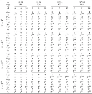
Table 2.Maximal theoretical regular circuit depths ofFV(DO) with the approximation

encoding, the CLPX approach encrypting the real and imaginary parts separately (DM),ComFVwith the approximation encoding (DA) and the fractional encoding (DF)

depending on input size (U), number of additions per level (A),nandq. Corresponding tandb’s are provided.

n 4096 8192 16384 32768

logq 116 226 435 889

A 0 3 10 0 3 10 0 3 10 0 3 10

U

=

2

8

DO 1 0 0 1 1 1 2 2 1 3 3 2

tO 234 − − 234 240 254 268 286 254 2135 2177 2128

DM 4 3 3 9 8 6 12 12 11 15 14 14

bM 2 2 2 23 22 2 29 29 25 233 217 217

DA 5 4 3 9 8 6 11 11 10 14 13 12

bA 22 22 22 26 24 22 210 212 210 234 224 220

DF 5 4 3 9 8 7 11 11 10 14 14 13

bF 2 2 2 25 23 22 29 29 28 233 233 229

U

=

2

16

DO 1 0 0 1 1 1 2 2 1 3 3 2

tO 234 − − 234 240 254 267 285 254 2134 2176 2127

DM 4 3 3 9 8 6 12 12 11 14 14 14

bM 2 2 2 23 22 2 29 29 25 218 218 218

DA 5 4 3 9 8 6 11 11 10 14 13 12

bA 22 22 22 26 24 22 210 212 210 234 224 220

DF 5 4 3 9 8 7 11 11 10 14 13 12

bF 2 2 2 25 23 23 29 212 210 234 223 219

U

=

2

32

DO 0 0 0 1 1 1 1 1 1 2 2 2

tO − − − 265 271 285 265 271 285 2130 2148 2190

DM 4 3 3 8 8 6 11 11 10 14 14 13

bM 2 2 2 23 23 2 29 29 25 234 234 217

DA 5 4 3 8 8 6 11 10 9 13 13 12

bA 22 22 22 26 26 22 218 210 28 234 240 228

DF 5 4 3 8 8 6 11 10 9 13 13 12

bF 22 2 2 25 25 22 217 210 27 233 239 227

U

=

2

64

DO − − − 0 0 0 1 1 1 2 1 1

tO − − − − − − 2129 2135 2149 2258 2135 2149

DM 4 3 3 8 7 6 10 10 10 13 13 12

bM 2 2 2 25 23 22 29 29 29 233 233 217

DA 4 4 3 7 7 6 10 10 9 12 12 11

bA 22 22 22 26 26 24 218 218 212 234 236 222

DF 4 4 3 7 7 6 10 10 9 12 12 11

bF 22 22 2 25 25 23 217 218 211 233 236 222

existing solutions encrypting complex numbers. As a result, for the same cipher-text modulusqand degreen, we can homomorphically evaluate between 5 and 12 times deeper circuits compared to existing solutions based on FV and na-tively encoding complex numbers. In comparison to the state of the art, which encrypts the real and imaginary parts of the complex numbers separately, our method reduces the size of ciphertexts by a factor of 2 making our scheme at least twice as efficient in time and three times more efficient in space.

References

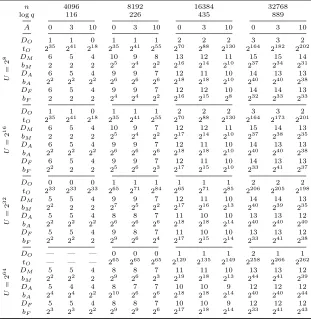
Table 3. Maximal heuristic regular circuit depths of the original FV scheme with native complex inputs (DO), the CLPX approach encrypting the real and imaginary

parts separately (DM),ComFVwith the approximation encoding (DA) and the fractional

encoding (DF) depending on input size (U), number of additions per level (A),nand

q. A correspondingtorbis provided.

n 4096 8192 16384 32768

logq 116 226 435 889

A 0 3 10 0 3 10 0 3 10 0 3 10

U

=

2

8

DO 1 1 0 1 1 1 2 2 2 3 3 2

tO 235 241 218 235 241 255 270 288 2130 2164 2182 2202

DM 6 5 4 10 9 8 13 12 11 15 15 14

bM 2 2 2 25 24 22 216 214 210 237 234 231

DA 6 5 4 9 9 7 12 11 10 14 13 13

bA 22 22 22 26 26 26 218 218 210 240 240 238

DF 6 5 4 9 9 7 12 12 10 14 14 13

bF 2 2 2 24 24 22 216 215 28 232 233 233

U

=

2

16

DO 1 1 0 1 1 1 2 2 2 3 3 2

tO 235 241 218 235 241 255 270 288 2130 2164 2173 2201

DM 6 5 4 10 9 7 12 12 11 15 14 13

bM 2 2 2 25 24 22 217 214 210 237 238 235

DA 6 5 4 9 9 7 12 11 10 14 13 13

bA 22 22 22 26 26 26 218 218 210 240 240 238

DF 6 5 4 9 9 7 12 11 10 14 13 13

bF 22 2 2 25 26 23 217 215 210 233 241 237

U

=

2

32

DO 0 0 0 1 1 1 1 1 1 2 2 2

tO 233 233 233 265 271 284 265 271 285 2206 2205 2198

DM 5 5 4 9 9 7 12 11 10 14 14 13

bM 22 2 2 27 25 22 217 216 213 240 239 235

DA 5 5 4 8 8 7 11 10 10 13 13 12

bA 22 22 22 26 26 26 218 218 214 240 240 240

DF 5 5 4 9 8 7 11 10 10 13 13 12

bF 22 22 2 29 26 24 217 215 214 233 241 238

U

=

2

64

DO — — — 0 0 0 1 1 1 2 1 1

tO — — — 265 265 265 2129 2135 2149 2258 2266 2262

DM 5 5 4 8 8 7 11 11 10 13 13 12

bM 22 22 2 29 26 23 219 218 213 244 241 239

DA 5 4 4 8 7 7 10 10 9 12 12 12

bA 24 24 22 210 26 26 218 218 214 240 240 244

DF 5 5 4 8 8 7 10 10 9 12 12 12

bF 23 23 22 29 29 26 217 218 214 233 241 243

encrypted data (2017), cryptology ePrint Archive: Report 2017/857

2. Bonte, C., Bootland, C., Bos, J.W., Castryck, W., Iliashenko, I., Vercauteren, F.: Faster homomorphic function evaluation using non-integral base encoding. In: CHES 2017. LNCS, vol. 10529, pp. 579–600. Springer, Heidelberg (Sep 2017) 3. Bos, J.W., Castryck, W., Iliashenko, I., Vercauteren, F.: Privacy-friendly

forecast-ing for the smart grid usforecast-ing homomorphic encryption and the group method of data handling. In: AFRICACRYPT 17. LNCS, vol. 10239, pp. 184–201. Springer, Heidelberg (May 2017)

4. Brakerski, Z., Gentry, C., Vaikuntanathan, V.: (Leveled) fully homomorphic en-cryption without bootstrapping. In: ITCS 2012. pp. 309–325. ACM (Jan 2012) 5. Chen, H., Laine, K., Player, R.: Simple encrypted arithmetic library - SEAL v2.1.

6. Chen, H., Laine, K., Player, R., Xia, Y.: High-precision arithmetic in homomorphic encryption. In: Smart, N.P. (ed.) CT-RSA 2018. LNCS, vol. 10808, pp. 116–136. Springer, Heidelberg (2018)

7. Cheon, J.H., Jeong, J., Lee, J., Lee, K.: Privacy-preserving computations of pre-dictive medical models with minimax approximation and non-adjacent form. In: FC 2017. vol. 10323, pp. 53–74. Springer, Heidelberg (2017)

8. Cheon, J.H., Kim, A., Kim, M., Song, Y.S.: Homomorphic encryption for arith-metic of approximate numbers. In: ASIACRYPT 2017, Part I. LNCS, vol. 10624, pp. 409–437. Springer, Heidelberg (Dec 2017)

9. Costache, A., Smart, N.P.: Which ring based somewhat homomorphic encryption scheme is best? In: CT-RSA 2016. LNCS, vol. 9610, pp. 325–340. Springer, Hei-delberg (Feb / Mar 2016)

10. Costache, A., Smart, N.P., Vivek, S.: Faster homomorphic evaluation of discrete Fourier transforms. In: FC 2017. LNCS, vol. 10322, pp. 517–529 (2017)

11. Costache, A., Smart, N.P., Vivek, S., Waller, A.: Fixed-point arithmetic in SHE schemes. In: SAC 2016. LNCS, vol. 10532, pp. 401–422. Springer, Heidelberg (Aug 2016)

12. Dowlin, N., Gilad-Bachrach, R., Laine, K., Lauter, K., Naehrig, M., Wernsing, J.: Manual for using homomorphic encryption for bioinformatics. Tech. rep., MSR-TR-2015-87, Microsoft Research (2015)

13. Fan, J., Vercauteren, F.: Somewhat practical fully homomorphic encryption. Cryp-tology ePrint Archive, Report 2012/144 (2012),http://eprint.iacr.org/2012/ 144

14. Geihs, M., Cabarcas, D.: Efficient integer encoding for homomorphic encryption via ring isomorphisms. In: LATINCRYPT 2014. LNCS, vol. 8895, pp. 48–63. Springer, Heidelberg (Sep 2015)

15. Gentry, C.: Fully homomorphic encryption using ideal lattices. In: 41st ACM STOC. pp. 169–178. ACM Press (May / Jun 2009)

16. Gentry, C., Halevi, S., Smart, N.P.: Homomorphic evaluation of the AES circuit. In: CRYPTO 2012. LNCS, vol. 7417, pp. 850–867. Springer, Heidelberg (Aug 2012) 17. Hoffstein, J., Pipher, J., Silverman, J.H.: Ntru: A ring-based public key cryptosys-tem. In: Algorithmic Number Theory, Third International Symposium, ANTS-III. pp. 267–288. Springer, Heidelberg (1998)

18. Lauter, K., L´opez-Alt, A., Naehrig, M.: Private computation on encrypted genomic data. In: LATINCRYPT 2014. LNCS, vol. 8895, pp. 3–27 (Sep 2015)

19. Lyubashevsky, V., Peikert, C., Regev, O.: On ideal lattices and learning with errors over rings. In: EUROCRYPT 2010. LNCS, vol. 6110, pp. 1–23. Springer, Heidelberg (May 2010)

20. Naehrig, M., Lauter, K.E., Vaikuntanathan, V.: Can homomorphic encryption be practical? In: ACM Cloud Computing Security Workshop – CCSW. pp. 113–124. ACM (2011)

A

The canonical norm

This appendix closely follows Appendix A.5 of the ePrint version of [6].

LetK=_Q[X]/(f(X)) be a cyclotomic number field where, as usual,f(X) =

Xn_{+ 1 is the 2n-cyclotomic polynomial,na power of two. We denote the ring}

modulo an ideal (a). Ifais a natural numberRa=Za[X]/(f(X)) and we take

representatives of_Z/a_Zfrom the half-open interval [−a/2, a/2). For anya =P

iaiX

i _{∈ K, the infinity norm kak}

∞ is defined as maxi|ai|.

We denote byδRthe upper bound onkabk_∞/kak_∞· kbk_∞for anya, b∈R. This bound is calledthe expansion factor ofR. For a our ring of cyclotomic integers

R, the expansion factor is δR =n. Let ζ is a complex primitive 2n-th root of unity. We definethe canonical norm as

kakcan_∞ = a(ζ), a(ζ3), . . . , a(ζ2n−1)

_∞.

It is easy to check that the canonical norm satisfies

kak_∞≤ kakcan_∞ , ka+bkcan_∞ ≤ kakcan_∞ +kbkcan_∞ , kabkcan_∞ ≤ kakcan_∞ · kbkcan_∞ .

The last inequality implies that the canonical norm leads to tighter bounds than the infinity norm [19].

Canonical norm of random polynomials We will need to bound the canoni-cal norm of random polynomials whose coefficients are generated from a discrete Gaussian or uniform distributions. We follow a heuristic approach given in [16, A.5], which was already used in [9, 5, 6] for an analysis of the FV scheme.

Leta∈Rbe a polynomial such that its coefficients are chosen independently from some zero-mean distribution with standard deviation σ. For this purpose, we use the following distributions

– a discrete Gaussian distributionD(σ2_{) with PMF proportional to exp(−}|x|2

2σ2),

– the uniform distributionU3 over the ternary set{−1,0,1}, – the uniform distributionUq overZq,

– the uniform distributionUrnd over the interval (−1/2,1/2].

By the definition of the canonical norm, we need to compute a(ζi

2n). The

evaluationa(ζi_{) is the inner product between the coefficient vector ofaand the}

fixed vector 1, ζi_{, . . . , ζ}i(n−1)

, which has Euclidean norm√n. Hence, the ran-dom variablea(ζi

2n) has varianceV =σ2nby the Cauchy-Schwartz inequality.

When ai ← D(σ2_{) then the coefficients have variance ' σ}2 _{and thus the} variance of a(ζi

2n) isVD 'σ2n. Ifai ← U3 then the coefficients have variance 2/3 and thus the total variance is VU3 = 2n/3. By analogy, VUq . q

2_{n/12 as} theaihas variance roughly q2/12. Finally, the variance ofai ← Urndis equal to 1/12, so VUrnd =n/12.

Sincea(ζi

2n) is the sum of independently distributed complex variables, by

the law of large numbers it is distributed similarly to a complex Gaussian random variable of variance V. Therefore, given that erfc(6) '2−55_{, we can use 6}√_V as a high-probability bound ona(ζi

2n). Since in practicen≥212, this bound is

distributions above, we get

kakcan_∞ ≤6σ√n, ai← D(σ2),

kakcan_∞ ≤2√6n, ai ← U3,

kakcan_∞ ≤q√3n, ai← Uq,

kakcan_∞ ≤√3n, ai← Urnd.

We also need to bound the canonical norm of a product of two random polynomials a and b whose coefficients are independently sampled from zero-mean distributions with variances σ2

1, σ22, respectively. Writing the product ab mod (Xn+ 1) with relation to the power basis ofR, we obtain



 

a0 −an−1. . .−a1 ..

. ... ...

an−1 an−2 . . . a0 

 



 

b0 .. .

bn−1 

 =



 

g0 .. .

gn−1 

 .

Hence, the product coefficients are equal to

gk= k

X

i=0

aibk−i− n−1 X

i=k+1

aibk+n−i.

for anyk∈[0, . . . , n−1]. Since the coefficient distributions are independent and have zero mean, the product of any pairai, bjhas varianceσ21σ22and zero mean. Hence, the variance of each coefficientgkis equal tonσ12σ22. Following the above reasoning, the canonical norm ofg(ζi_{) is thus bounded by}

kabkcan_∞ ≤6nσ1σ2.

This means that the variance of the coefficients of ue where u ← χk and e ← χe is approximately 2σ2n/3. We can now give the variance of the term

appearing in the analysis of the decryption noise.