Eeg De-Noising Using Wavelet Transform And Fast Ica

EEG De-noising using Wavelet Transform and Fast ICA

Prof. Sachin Borse,

Department of Electronics and Telecommunication, Late G. N. Sapkal College of Engineering, Nashik

India

Abstract

The paper deals with the use of wavelet transform and Independent component analysis (ICA) for EEG signal de-noising using a selected method of thresholding of appropriate decomposition coefficients. The presented technique is based upon the analysis of wavelet transform and it includes description of global modification of its values. The whole method is verified for simulated signals and applied for processing of biomedical signals representing EEG signals can be used for MR images corrupted by additional random noise. In ICA method, ICA algorithm is applied to derive the independent components. The ICA components associated with artifactual events then cancelled out.

Keywords: WT, EEG, db4, sym4, ICA.

1. Introduction

The

wavelet transform

(WT) is a powerful tool

of signal processing for multi-resolution

analysis. WT is suitable for application to

non-stationary signals with transitory phenomena,

whose frequency response varies in time [2]. The

wavelet coefficients shows similarity in the

frequency content between a signal and a chosen

wavelet function [2]. These coefficients are

computed as a convolution of the signal and the

scaled wavelet function, which can be

interpreted as a dilated band-pass filter because

of its band-pass like spectrum [5]. The

scale

is

inversely proportional to radian frequency.

Consequently, low frequencies correspond to

high scales and a dilated wavelet function. By

wavelet analysis at high scales, we extract global

information from a signal called

approximations

.

Whereas at low scales, we extract fine

information from a signal called

details

. Signals

are usually band-limited, which is equivalent to

having finite energy, and therefore we need to

use just a constrained interval of scales.

However, the continuous wavelet transform

provides us with lots of redundant information.

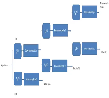
The

discrete wavelet transform

(DWT) requires

less space utilizing the

space-saving coding

based on the fact that wavelet families are

orthogonal or bi-orthogonal bases, and thus do

not produce redundant analysis. The DWT

corresponds to its continuous version sampled

usually on a

dyadic

grid, which means that the

scales and translations are powers of two [5]. In

practice, the DWT is computed by passing a

signal successively through a high-pass and a

low-pass filter. For each decomposition level,

the high-pass filter

hd

forming the wavelet

function produces the

approximations A

. The

complementary low-pass filter

ld

representing

the scaling function produces the

details D

[3].

This computational algorithm shown in Figure 1

is called the

subband coding

.

The filtering

process changes the resolution and also the scale

is changed by up sampling and down

sampling process.

This is given as

(1)

Fig. 1 Sub band coding for EEG de-noising. The synthesis filtering consists of up sampling by 2 and filtering.

(3)

Reconstruction filters attain to produce the perfect signal reconstruction from the DWT coefficients on condition that the signal is of finite energy and satisfies the admissibility condition. In this application we used Daubeschies wavelet db4.

2. Signal Analysis

Wavelets are used for wide variety of applications, like de-noising, detecting the features, breakdown points, and discontinuities etc. We focus on discontinuity detection. Wavelet analysis is a time frequency analysis. It has capacity of representing local characteristics in time and scale domains. More features can be understood as it has capability of transforming the time domain signal in time frequency localization. In low frequency, it has lower time resolution and in high frequency, it has higher time resolution and lower frequency resolution.

The discrete wavelet transform (DWT) decomposes the signal into two phases: detail and approximation data on different scales. The approximation domain is sequentially decomposed into further detail and approximation data. These decompositions of the signal can act as the input matrix for ICA technique. The DWT means choosing subsets of the scales ‘a’ and positions ‘b’ of the mother wavelet ψ (t).

Ψ(a,b)(t) = 2a/2 Ψ(2at-b)

(4)

Here, the mother wavelet functions are dilated by powers of two and translated by integers. Scales and positions chosen based on power of two are named as dyadic scales and positions. The discrete wavelet transform does not preserve the translation invariance. To preserve the translation invariance property, a new approach has been defined as stationary wavelet transform (SWT) which is close to the DWT one.

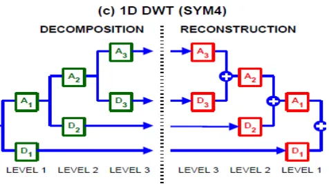
For the Electroencephalogram (EEG) signal, Fig.1 demonstrates the use of db4 wavelet to remove the noise and discontinuities. Db4 is chosen as it suits with the input signal which is EEG in this case. Three level decomposition is used which is enough to make the discontinuity apparent.

3. EEG Signal De-noising

3.1 Soft and Hard thresholding

In signal de-noising there are three successive procedures, namely signal decomposition thresholding of the DWT coefficients and signal reconstruction. In first step, we carry out wavelet analysis on noisy signal up to chosen level N in our case 3. In second step we perform thresholding of the detail coefficients from level 1 to N. Lastly the signal synthesized using altered detail coefficients from level 1 to N.

For thresholding, we settle either a level dependent threshold vector of length N or a global threshold of a constant value for all levels. The threshold estimate for de-noising using D. Donoho’s method is given by

(5)

Where the noise is Guassian with standard deviation Of the DWT coefficients and L is the number of samples or pixels of processed signal or image.

Thresholding can be either soft or hard[1]. All the signal values smaller than are zeroed out. In Soft thresholding it subtracts from the values larger than . Soft thresholding does not cause discontinuities in the resulting signal.

3.2 Applications of EEG signal

De-noising is shown in Fig 2. Thresholding of the DWT coefficients up to level 3 is used to remove the random noise. As a wavelet function we chose sym4 as it performs better than db4. We used soft global threshold of an estimated value given by equation [5].

The code is as given below.

eeg=load('EEG01.TXT');

eeg=detrend(eeg); % Remove a linear trend eeg=eeg(100:611);

L=length(eeg);

eegN=eeg+160*randn(L,1);

[THR,SORH,KEEPAPP]=ddencmp('den','wv',eegN); level=3;

[eegC,CeegC,LeegC,PERF0,PERFL2]=wdencmp('gbl',eeg N,'sym4',level,THR,SORH,KEEPAPP);

Fig. 2 Decomposition and Reconstruction.

The original noisy signal is as shown in Fig. 3.

Fig.3 Original Noisy Signal

The clean EEG signal is as shown in Fig. 4.

Fig. 4 Clean EEG output using ‘sym4’.

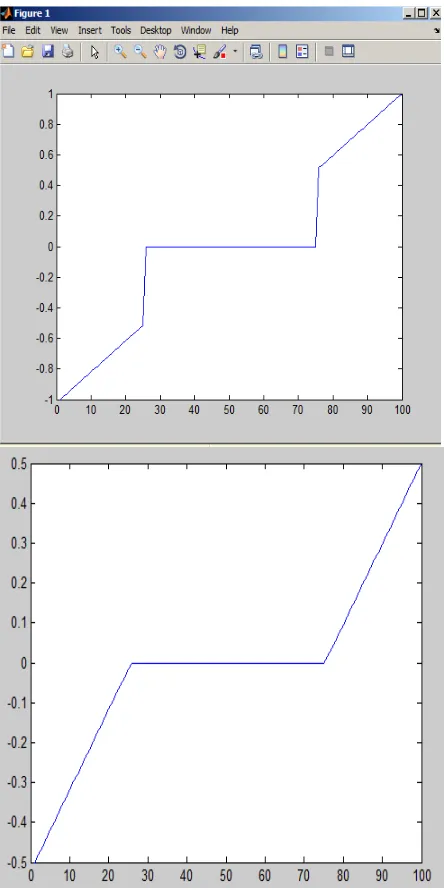
To calculate the threshold the following code

can

eeg=load('EEG01.TXT');

eeg=detrend(eeg); % Remove a linear trend eeg=eeg(100:611);

eeg = linspace(-1,1,100); thr = 0.5;

eegthard = wthresh(eeg,'h',thr); plot(eegthard);

eegtsoft = wthresh(eeg,'s',thr); plot (eegtsoft);

Fig. 5. Shows Hard thresholding and Soft thresholding.

Fig. 5 Hard Thresholding(Above) and Soft Thresholding(Below)

Along with hard thresholding in many applications soft thresholding procedures are often used. The only difference between the hard and the soft thresholding procedures is in the choice of the nonlinear transform on the empirical wavelet coefficients.

4.

EEG Signal Denoising Using ICA

In this work, before applying ICA random

noise is added in a raw EEG signal. ICA is

applied to this noise mixed signal. ICA is

powerful technique to separate the independent

sources linearly mixed in several sensors. In this

work ICA is used to remove the linearly mixed

noise from the original EEG signal. When

recording Electroencephalogram (EEG) on the

scalp, ICA can separate out artifacts embedded

in the data.

Two raw EEG signals are used and noise

is mixed in both the signals. The look like as

shown in Fig. 6.

4.1 Whitening the Data

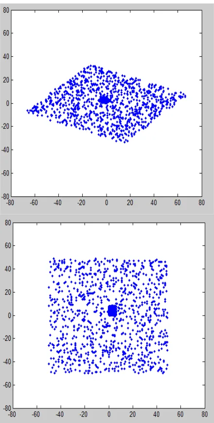
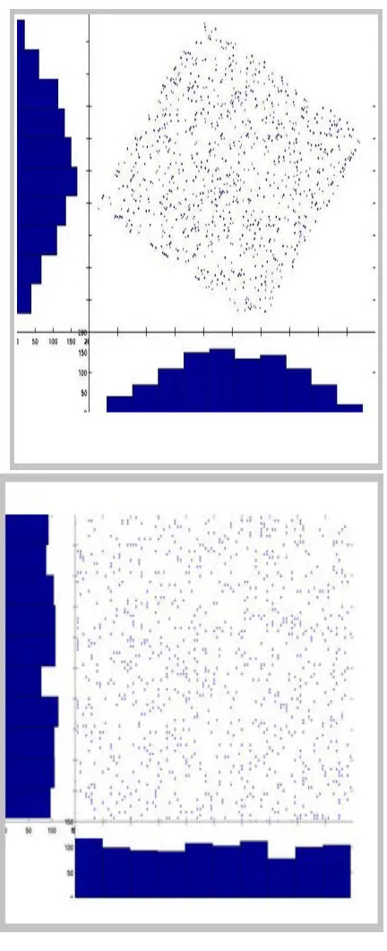
Whitening is the process performed by most ICA alogorithms before applying the actual ICA. This is the first step in many ICA algorithm. It removes the correlation present in the data i.e. different channels are uncorrelated. The reason behind doing this is a geometrical interpretation is that it restores the initial shape of the data and that then ICA must only rotate the resulting matrix. One more time the two raw EEG signals(sat A and B) are mixed, at each time A is abscisia of the data point and value of B is their ordinates as shown in Fig. 7.

Fig. 7 Plot of Linearly mixed variables.

Fig. 8 shows the whitened variable of two linearly mixed signals.

Fig. 8 Whitened data

The variance on both the axis is equal and the correlation of the projection of the data on both the axis is 0. It means that the covariance matrix is diagonal and that all the diagonal elements are equal. Then apply ICA, it is process of rotating this representation back to the original A and B axis space.

The whitening process is a linear change of coordinate of the mixed data. Once the ICA solution is found in this whitened coordinate frame one can easily reproject the ICA solution back into the original coordinate frame.

4.2 ICA Process

Fig. 9 Fixed point ICA

The projection on both the axis is quite Guassian. By rotating the axis and minimizing Gaussianity of the projection in the first scatter plot, ICA is able to recover the original sources which are statistically independent.

5. Conclusions

This work provides practical example of EEG signal denosing and signal improvement using the wavelet transform along with the enclosed Matlab code. The data we processd is a real biomedical ECG signal. This method based on wavelet analysis for removal of noise or artifacts from EEG may lead to loss of the data and there may be still remnant artifact in the collected samples and further investigation can be easily done by comparing this data with data obtained by invasive methods.

For ICA analysis two random signals are generated and they are mixed with noise. ICA algorithm shows that it is efficient method to separate multiple signals from noise as well as from each other.

References

[1] T. Nguyen G. Strang. Wavelets and Filter Banks. Wellesley-Cambridge Press, 1996.

[2] G. Oppenheim J. M. Poggi M. Misiti, Y. Misiti. Wavelet

Toolbox. The MathWorks, Inc.,

Natick, Massachusetts 01760, April 2001.

[3] S. Mallat. A Wavelet Tour of Signal Processing. Academic Press, San Diego, USA, 1998.

[4] R. Polikar. Wavelet tutorial. eBook, March 1999. http://users.rowan.edu.

[5] C. Valens. A really friendly guide to wavelets. eBook, 2004. http://perso.wanadoo.fr.

[6] E. W. Weisstein. Mathworld. eBook, 2003. http://mathworld.wolfram.com.

[7] Amod Kumar, Wavelet-ICA based Denoising of Electroencephalogram Signal, International Journal of Information & Computation Technology. ISSN 0974-2239 Volume 4, Number 12 (2014), pp. 1205-1210.

[8] M. Teplan Fundamentals of EEG measurement Measurement Science Review, 2002; Vol. 2 (2)

[9] Aapo Hyvärinen, Erkki Oja Independent component analysis: algorithms and applications Neural Networks, 2000; 13: 411-430

[10] Ganesh R. Naik, Dinesh K Kumar An overview of independent component analysis and its application Informatica 2011; 35: 63-81