TEXT INTERPRETATION USING A MODIFIED PROCESS
OF THE ONTOLOGY AND SPARSE CLUSTERING
1
IONIA VERITAWATI, 2ITO WASITO, 3T. BASARUDDIN
1
Lecturer, Department of Informatics, University of Pancasila, Srengseng Sawah, Jakarta, Indonesia
2
Assoc. Prof., Faculty of Computer Science, University of Indonesia, Kampus UI Depok, Depok, Indonesia
3
Prof., Faculty of Computer Science, University of Indonesia, Kampus UI Depok, Depok, Indonesia
E-mail: [email protected], [email protected], 3chan@ cs.ui.ac.id
ABSTRACT
Many texts in online media consist of various information that need an appropriate way to extract and interpret them clearly. For better understanding of the content in the text collected from any online media, a proper methodology for the interpretation of useful information must be developed. This study offers a modified process of the text interpretation consisting of four stages with a preliminary stage of the text preprocessing and key phrase extraction using the annotated suffix tree (AST) technique and secondary stage of developing sparse clustering method named as iterative scaling of fuzzy additive spectral clustering (is-FADDIS) combined with a sharpening technique for grouping key phrases from the text. An ontology as the “knowledge base” was developed combining with is-FADDIS method as the third stage. Interpretation from the input text was carried out as the final stage of the text interpretation. The performances of is-FADDIS clustering combined with sharpening technique as high as 96 and 78% were verified for some modeled sparse data and two specific real sparse data from two corpus, respectively, and could be better when comparing with Nonnegative Matrices Factorization (NMF) and K-means. The text interpretation of using the ontology gives a clear graph visualization on the relationship among key phrases even though it has a low correlation with content of the text. The result findings of this study potentially help us in ensuring an automatic process to be used for the interpretation of any topic information collected from online media.
Keywords: Annotated Suffix Tree, is-FADDIS, Ontology, Sparse Clustering, Text Interpretation
1.
INTRODUCTIONText mining as a methodology to process the content of text collection becomes popular to help people extracting the information and knowledge. It includes text preprocessing, clustering, classifying and others. Ontology can be included in text mining to give specific result in extraction of information.
Text interpretation is a part of text mining which explores content of text. The examples applied, such as text interpretation are changed to become motion language as avatar animation [2], to translate language using dictionary [3], to mine useful patterns in text documents [1]. Besides, it is also used to interpret words based on Latent Semantic Similarity in vector space model, using WordNet and Google Distance by ranking the results [4], to help for understanding context of a text collection, such as news, scientific journals [5], to do a fast process of information for a decision-making [6], to analyze topics for seeing the trend of
customer needs in a specific domain; such as banking [7], to understand knowledge from domain of biomedics [8], and others.
Fayyad, et. al [9] developed a framework to discover knowledge that can be interpreted. Data mining is applied to get the concept (key word) from electronic articles in a database. Vectors data from the key words are transformed to find patterns so that knowledge in an article can be extracted.
Adaptation is done by O'Callaghan [10] based on framework Fayyad et al., in which the results of data mining are compared with expert opinion. The results of the data mining process are a grouping topic of a dataset journal. The advantages of the framework generates journal data grouping significantly while the disadvantages of such research do not use full text, as there are a lot of features and noise.
reference in a text interpretation. It can also be used to assist extracting knowledge in the collection of documents [11] and the expert system guided by ontology to recommend a good or bad knowledge [12]. Another research using clustering technique and ontology reference are used by Mirkin et. al [13] to gain knowledge from research activities in an organization. These show that ontology has advantages that encapsulate domain knowledge in the form of concepts and their relationships in a structure. It can give more meaningful information when performed extracts on different domains.
From various interpretations and objects interpreted, text interpretation has a great opportunity to be studied. The proposed method is a text interpretation based on key phrases using ontology and sparse clustering in a text collection.
2.
BACKGROUNDThis section discusses about text preprocessing, spectral clustering, sparse clustering and ontology concept.
2.1.Preprocessing and Key Phrase Extraction
Collection of text can be from documents, articles, books and others. Text is a collection of words such as basic words, affix words and stop words. It is powerful to communicate ideas, information, knowledge and others. In text processing, it needs to extract key phrases contained in the text, as main elements.
Text Preprocessing is applied to the text for removing stop words, stem [14] affix words and extract key phrases (KP) using AST (Annotated Suffix Tree) which KPs can consist of one or more words. After that, a table or a matrix of frequencies, key phrases versus documents is developed [15]. A normalization process using tf-idf is applied to the matrix from text data. The normalization is whose the frequencies of key phrases are multiplied by invers log of existence of each key phrase in a document.
2.2.Spectral Clustering
Clustering is one important process to be applied in grouping the text to be become several topics or domains. It has more specific information so that it can be more understandable. There are several approaches of clustering methods including hard clustering and soft (fuzzy) clustering. Another type of clustering is spectral clustering which processes a vector of data in Vector Space Model (VSM) by converting it to eigen space which consists of eigen
values and eigen vector as a basis element of data. As a result, the data can be ranked according to the eigen values. Six dominant eigen vectors related to eigen values can be chosen as data representing the data [16].
This experiment uses spectral clustering which is modified from Fuzzy Additive Spectral Clustering (FADDIS) and it belongs to fuzzy clustering. FADDIS is applied to different types of data including affinity data, community structure, and others [17]. Algorithm of FADDIS processes similarity of data using Gaussian similarity to make up affinity data. The data convert to eigen space, and the maximum eigen values are chosen to calculate Rayleigh Quotient (RQ). The value from RQ is used to calculate contribution value of the maximum eigen values and calculate the residual of affinity data. The residual is processed in the same way iteratively until the contribution value is close to zero. The process is called fuzzy because the clustering output is memberships of data in each cluster.
2.3. Sparse Clustering
In area of text mining, data matrix is developed from feature data usually in sparse condition. Sparse data is a data which is dominated by zeros. After the text preprocessing, the matrix resulted is a sparse data. Because key phrases are unique words which depend on domain, the frequencies do not always exist in all documents.
Non Negative Matrices Factorization (NMF) is one method that can be used to process a sparse matrix to cluster documents [18]. Besides, modified K-means as a popular method can be used to cluster a sparse matrix [19]. Other methods, the combination of Non-negative and Sparse Spectral Clustering can be applied to sparse data [20].
2.4.Ontology Concept
Ontology is broadly defined as “a formal, explicit specification of a shared conceptualization”[21]. Generally, the representation of domain ontology has spectrum ranging from lightweight ontology whose the structure is represented by a taxonomy (tree or graph) to formal ontology represented by a relational data base [22].
3.
PROPOSED METHOD3.1. Methodology
presented (figure 1). Ontology is developed from a text or document collection. An inputted text is interpreted using the ontology and will give a graph visualization of key phrases related to the inputted text.
Figure 1: Illustration of Methodology for Text Interpretation
3.2. A New Sparse Clustering
For clustering a sparse data, FADDIS (algorithm 1) cannot be used because it works into data with normal distribution. A proposed method for clustering called iterative scaling-Fuzzy Additive Spectral (is-FADDIS) is presented (algorithm 2). It is a modification algorithm as iterative process using FADDIS in each iteration, and using scale as well as internal validation as a stop criterion. The clustering technique applied to sparse data is combined by a sharpening technique which adds noises to original data according to two thresholds for key phrase and document.
3.3. Ontology Development
Figure 2: Method of Ontology Development
Method of ontology development consists of several steps (figure 2). It is built from a corpus. The process is started with preprocessing, extracting key phrase and building a vector data. It is followed by clustering [23]. Is-FADDIS as a sparse clustering is applied to the vector data which functions to separate its data elements. The
clustered data are categorized and then they become input data for structure learning process using bayesian network. A scoring function, Markov Chain Monte Carlo (MCMC) method, is applied to each clustered data to predict a graph structure (sub-Ontology). After connector analysis process and tree ontology development, the result is visualized as an ontology model.
3.4. Text Interpretation
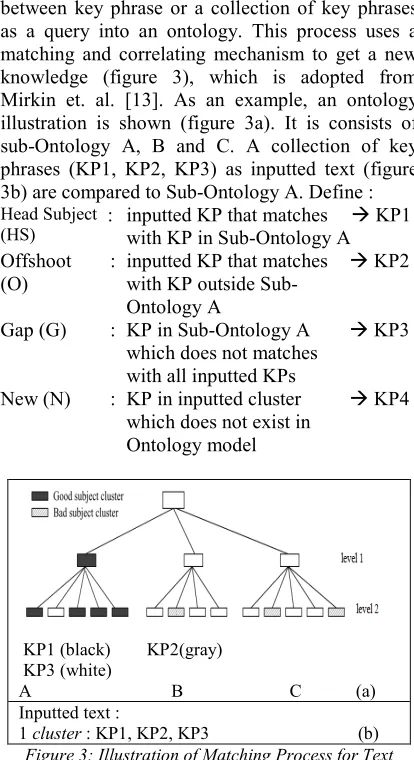
Text interpretation is an extracting process between key phrase or a collection of key phrases as a query into an ontology. This process uses a matching and correlating mechanism to get a new knowledge (figure 3), which is adopted from Mirkin et. al. [13]. As an example, an ontology illustration is shown (figure 3a). It is consists of sub-Ontology A, B and C. A collection of key phrases (KP1, KP2, KP3) as inputted text (figure 3b) are compared to Sub-Ontology A. Define : Head Subject
(HS)
: inputted KP that matches with KP in Sub-Ontology A
KP1
Offshoot (O)
: inputted KP that matches with KP outside Sub-Ontology A
KP2
Gap (G) : KP in Sub-Ontology A which does not matches with all inputted KPs
KP3
New (N) : KP in inputted cluster which does not exist in Ontology model
KP4
KP1 (black) KP2(gray) KP3 (white)
A B
C (a) Inputted text : [image:3.612.313.520.228.608.2]
1 cluster : KP1, KP2, KP3 (b) Figure 3: Illustration of Matching Process for Text
[image:3.612.86.303.493.627.2]Interpretation [13] (a) Ontology (b) inputted text;
Table 1. Matching table from 1 of Text Cluster to the Ontology
Sub Onto logy
HS = matching Score
Off-shoot Gap New Total cluster
1 2 3 4 1+2+3
A X % Y % - Z% (X+Y+Z) %
score, which total is 100% (table 1). The matching score used is HS score (column 1).
An ontology model as a “knowledge base” in Indonesian language is defined (figure 4a), which inputted cluster (figure 4b) will be matched. For this example, text KPclust(1) is to be matched and correlated. It results a graph visualization, “interpretation 1” (figure 4c), and a matching score (table 2, column 1), which matches with sub-Ontology A as the biggest HS score (matching score), compared to the HS score of sub-Ontology B and C. For text cluster KPClust(2), with the same process, the matching result is sub-Ontology C, and the result information is “interpretation 2” (figure 4c).
A B C (a) KPclust{1}={ 'buah' 'apel' 'nangka' 'nanas' 'pepaya'} (='fruit' 'apple' 'jackfruit' 'pineapple' 'papaya') KPclust{2}={'salam' 'bawang merah' 'wortel'} (='salam' 'red onion' 'carrot') (b)
(c)
Interpretation1 Interpretaion 2
Figure 4: (a) Ilustration of Text Interpretation using Ontology ; (b) Inputted text
Table 2. Matching Table of Text Cluster 1 - KPclust(1)
Sub
Onto-logy HS-matching score (%)
Offshoot (%)
Gap (%)
New (%)
Total cluster (%) (1) (2) (3) (4) (1)+ (2)+(3)
A 60 0 40 40 100
B 0 60 100 40 100
C 0 60 100 40 100
4.
RESULTS AND DISCUSSIONThe experiments consist of two parts. The first part is experiment of sparse clustering from vector data. The second part is applied text interpretation
from inputted text using ontology, as presented in methodology of text interpretation (figure 1).
4.1. Sparse Clustering Result
The first part of experiments uses various sparse clustering methods. These include FADDIS or scaling-FADDIS (s-FADDIS), NMF, is-FADDIS, also K-means and Hierarchical Clustering (HC). The methods are applied to modeled vector data consist of one normal distribution data and four sparse data with different sparsities. The methods are also applied to three vector data from UCI dataset consisting of Bupa, Glass, CNAE, and two real data of corpus. Validation methods to the clustering results use Silhouette and Davies Bouldin (DB) index for internal validation. Purity and Adjusted Rand Index are used for external validation.
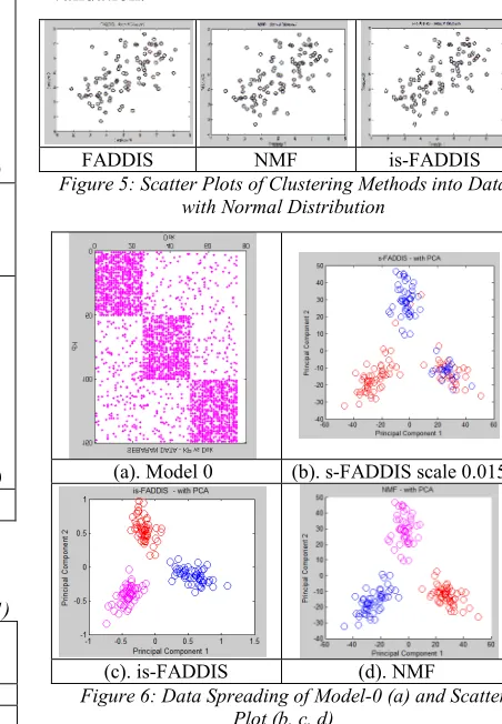
[image:4.612.91.526.279.650.2]FADDIS NMF is-FADDIS
Figure 5: Scatter Plots of Clustering Methods into Data with Normal Distribution
(a). Model 0 (b). s-FADDIS scale 0.015
(c). is-FADDIS (d). NMF Figure 6: Data Spreading of Model-0 (a) and Scatter
Plot (b, c, d)
[image:4.612.290.516.304.630.2]give the highest score of validation (table 3, row 3 and 5).
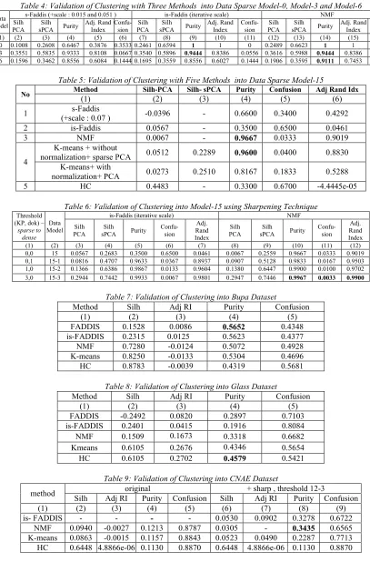
s-FADDIS is a basic method of is-FADDIS which uses a constant value for scaling data values. It is applied to sparse data (three clusters) model-0; with sparsity is 0.63 (figure 6a). The scatter plot result of s-FADDIS (figure 6b) shows that separation of data is not clear. is-FADDIS and NMF method are also applied to the modeled data. NMF as a well-known method is used to compare the clustering result of is-FADDIS as a proposed method. The results using is-FADDIS (figure 6c) and NMF (figure 6d) present a well separated data. iFADDIS method, as an iterative process of s-FADDIS, can cluster the data, with almost similar separation result compared to NMF method. Internal and external validation results of model-0 (table 4, row 1) show that purity of is-FADDIS and NMF are 1 and purity of s-FADDIS is 0,647. Silhouette, Adjusted Rand Index and Confusion of is-FADDIS and NMF also give higher values compared to s-FADDIS, and almost similar values between them.
The next modeled of sparse vector data which have three clusters are model-3, model-6 and model-15 (figure 7a, 7b, 7c). The spreading of all the modeled data show the sparsity of data which values are 0.71, 0.62, 0.83 respectively.
(a) Model-3 (b) Mode-6 (c) Model-15
Figure 7: Spreading of Data Sparse Model
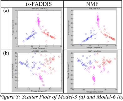
s-FADDIS, Is-FADDIS and NMF methods are applied to model-3 (figure 7a). The scatter plots of clustering results from is-FADDIS (figure 8a, column 1) and NMF (figure 8a, column 2) show almost the same well separated data. Internal and external validation of these clustering (table 4, row 2, column 7-16) still show almost the same values. Meanwhile, all validation values from s-FADDIS with appropriate scale (table 4, row 2, column 2-6) are comparable to is-FADDIS and NMF.
s-FADDIS, is-FADDIS and NMF methods are also applied to model-6 (figure 7b). The scatter plots of clustering results from is-FADDIS (figure
8b, column 1) and NMF (figure 8b, column 2) show the separation of data from the two methods are almost well separated. Internal and external validation of from NMF clustering result (table 4, row 3, column 12-16) show higher values compared to is-FADDIS results (table 4, row 3, column 7-11). Meanwhile, all validation values from s-FADDIS with appropriate scale (table 4, row 3, column 2-6) give almost the same values compared to is-FADDIS.
is-FADDIS NMF
(a)
(b)
Figure 8: Scatter Plots of Model-3 (a) and Model-6 (b) using is-FADDIS and NMF
s-FADDIS clustering results, with appropriate scale, into model 3 and model 6 give almost the same validation values compared to validation values from is-FADDIS. Is-FADDIS is used to be compared with NMF. It means, for model 3 and 6, as semi sparse data, is-FADDIS still does the clustering well, meanwhile FADDIS does not run well.
(a) s-FADDIS
scale 0.07 (b) is-FADDIS (c) NMF
(d) Kmeans + normalization +
PCA
(e) Kmeans +without normalization + sparse PCA
[image:5.612.320.516.214.376.2](f) HC
Figure 9: Scatter Plots of Data Model-15, using Five Methods of Clustering
model-15 (figure 7c). The clustering results of model-15 shows different separated data (figure 9). The results from NMF (figure 9c) and K-means (figure 9d, figure 9e) gives the best separation. Purity from external validation values using NMF and k-means (without normalization) are about 0.96 (table 5; row 3, 4), meanwhile s-FADDIS, is-FADDIS and HC give poor purity values (table 5; row 1, 2, 5). It means is-FADDIS and HC does not work well in clustering for spreading data with overlap, and s-FADDIS need an appropriate scale to work well.
A sharpening technique is proposed to overcome clustering whose data overlaps (algorithm 3). The technique adds noise values to the sparse data matrix to make the sparse data denser. It uses thresholds of key phrases (thresKP) and document (thresDok) in each non zero sparse data. The sharpening technique is applied into data model-15 (figure 10). It uses different thresholds to make spreading of data model-15 denser (model 15-1, model 15-2 and model 15-3). Before the technique applied to model-15, is-FADDIS clustering result is not well separated (figure 11a). After applying the sharpening technique, the clustering results get a better separation (figure 11b, 11c, 11d).
Data Model 15-1 thres(KP,Dok)=0-1
Data Model 15-2 thres(KP,Dok)=1-0
Data Model 15-3 thres(KP,Dok)=3-0
[image:6.612.312.523.347.518.2]Figure 10: Data Model-15 + sharp: (a) threshold 0-1; (b) threshold 1-0; (c) threshold 3-0
model 15 model 15-1 model 15-2 model 15-3 thres 0-0 thres 0-1 thres 1-0 thres 3-0
(a) (b) (c) (d)
Figure 11: Clustering Results using is-FADDIS into Data Model-15 Combined with Sharpening Technique
Based on results from table 5, which NMF method gives the highest score of validation, the sharpening technique is also used by NMF to cluster the same data. External and internal validation clustering of different threshold of sharpening technique from model-15 using is-FADDIS and NMF shows that the highest validation values are in data model 15-3 with threshold combination 3-0 Table 6, row 4).
Validation results from is-FADDIS and NMF give almost the same values. The purities are about 0.99.
After applied clustering methods into modeled sparse data, the methods are applied to standard data UCI, Bupa, Glass and CNAE. Internal and external validation of clustering result into normalized Bupa shows that FADDIS and is-FADDIS give the best separation (table 7). Applying the same methods of clustering into normalized Glass, validation of clustering result using HC give the best values (table 8), so that FADDIS, applied to CNAE which is a sparse data. Commonly, the validation scores of clustering are low, but HC has good performance in clustering into Bupa and Glass as full data. Sharpening technique is using is-FADDIS, NMF, K-means and the sharpening technique to CNAE data give higher values than original data score (Table 9). Meanwhile, HC combined with the sharpening technique has no effect to clustering result of CNAE.
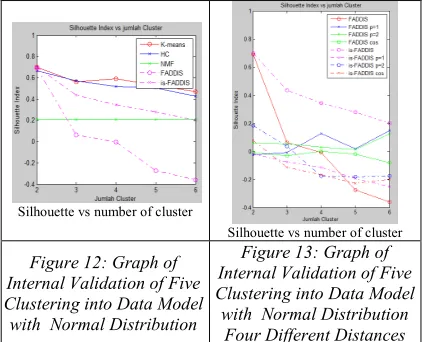
Silhouette vs number of cluster
Silhouette vs number of cluster
Figure 12: Graph of Internal Validation of Five Clustering into Data Model with Normal Distribution
Figure 13: Graph of Internal Validation of Five Clustering into Data Model with Normal Distribution Four Different Distances
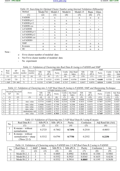
A visual of validation consists of graphs from five methods clustering (FADDIS, NMF, is-FADDIS, K-means, HC) into data (two clusters) with normal distribution is presented (figure 12). Each graph shows internal validation (silhouette index) values versus number of cluster. The maximum values of silhouette shows the optimal cluster number of data separation. It shows that all the clustering methods except NMF can show that the optimal cluster number is two clusters.
[image:6.612.88.302.404.603.2]Minkowski p=1 and p=2 can show that the optimal cluster number is two clusters.
Silhouette vs number of cluster
[image:7.612.89.300.122.301.2]Silhouette vs number of cluster Figure 14: Graph of
internal validation of five Clustering into Data
Sparse Model -3
Figure 15: Graph of Internal Validation of Five
Clustering into Data Sparse Model -3 - Four Different Distance
A visual of validation consists of graphs from five methods clustering (FADDIS, NMF, is-FADDIS, K-means, HC) into data (three clusters) with sparse – model-3 is presented (figure 14). Each graph shows internal validation (silhouette index) values versus number of cluster. It shows that NMF and can show that the optimal cluster number is three clusters.
The same type of graphs shows validation result of the similar four different distances which are applied to FADDIS and is-FADDIS for clustering the sparse data model-3 (figure 15). It shows that the clustering methods is-FADDIS with Gaussian distances almost can show that the optimal cluster number is three clusters.
The rest of modeled sparse data (6, model-15) and dataset UCI – Bupa and Glass are also tested to search the optimal cluster number. A sharpening technique combined with is-FADDIS is applied into the sparse modeled data.
The results of all graph plots are resumed (table 10). It shows the methods which fit cluster number of the data tested. Generally, FADDIS fits a full data or normal distribution data. Is-FADDIS with or without sharpening technique fit semi sparse or sparse data, as well as NMF, K-means sometimes fit full data or semi sparse data.
According to the experiment into sparse data model-15 (table 6), is-FADDIS combined with sharpening technique give almost the same result as NMF with sharpening threshold 3-0, a well-known method. Besides, comparing the clustering results into UCI dataset, is-FADDIS and NMF fit sparse data (CNAE), also determination of optimal cluster
number (table 10) which is-FADDIS and NMF are fit semi sparse or sparse data. Based on those results, is-FADDIS and NMF methods are applied into real data corpus, which is processed to become a sparse matrix before it is clustered.
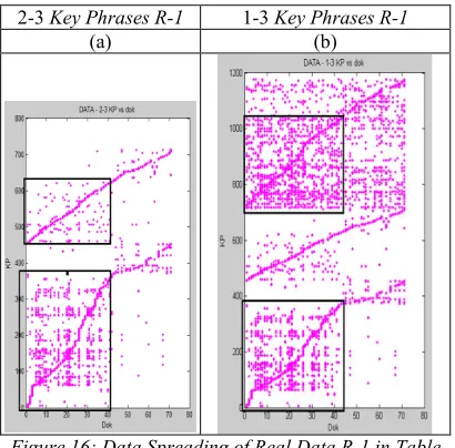
The first Real Data is data R-1. It is a corpus which uses an Indonesian text collection consisting of two domains of news, economy (40 documents) and sport (31 documents). The process to data R-1 is started from text preprocessing, followed by key phrase extraction using AST until development of matrix data. The spreading of matrix with non zeros values in shown (figure 16). Data matrix of R-1 is separated into 2-3 KP data (figure 16a) and 1-3 KP data (figure 16b). The scatter plots using is-FADDIS clustering into 2-3 KP and 1-3 KP are presented (figure 17a, column 1 and 2) and using NMF also into 2-3 KP and 1-3 KP are presented (figure 17b, column 1 and 2).
2-3 Key Phrases R-1 1-3 Key Phrases R-1
(a) (b)
Figure 16: Data Spreading of Real Data R-1 in Table Key Phrase versus Document
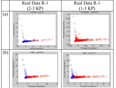
[image:7.612.316.521.322.524.2]According clustering results that 2-3 KP data gives better separated results, the next experiment only use the 2-3 KP data. The scatter plots into 2-3 KP data using is-FADDIS and NMF combined to sharpening technique in different thresholds is shown (figure 18). Is-FADDIS with sharpening technique into 2-3 KP data R-1 at thresholds 22-2, gives the highest validation value (table 12, row 7). At that threshold, is-FADDIS also has higher validation values compared to NMF with the same sharpening technique.
Real Data R-1 (2-3 KP)
Real Data R-1 (1-3 KP) (a)
[image:8.612.95.296.226.378.2](b)
Figure 17: Scatter Plots of Clustering using is-FADDIS (a) and NMF (b) into Real Data (2-3 KP) - 2 Cluster and
(1-3 KP)
(a) thresKP-thresDok :14-2 (b) thresKP-thresDok :20-2
(c) thresKP-thresDok:21-2 (d) thresKP-thresDok :22-2
noise value =max
Figure 18: Scatter Plots of Clustering using is-FADDIS and Sharpening Technique into Real Data Sparse 2-3 KP
Data with Different Thresholds
The results of clustering using K-means are presented (table 13). Before using sharpening technique, the validation results are better than using is-FADDIS (row a). After using sharpening technique (row b) with at thresholds 22-2, the validation values get better; but is-FADDIS with the same technique (table 12, row 7) gives a better validation. According to the comparison results, is-FADDIS with sharpening technique which gives
the best result of clustering will be used in ontology development into Real data R-2.
Time complexity of clustering algorithm K-means is O(nkT), HC is O(n3), FADDIS is O(n3), NMF is O(n3) and is-FADDIS is O(n4). It means, is-FADDIS needs more time compare to others, but potentially can separate data in sparse condition.
4.2. Ontology Development and Text
Interpretation
The second part of experiments is Text Interpretation. It is done using a corpus - Real Data R-2. This second Real Data is an Indonesian text collection consisting of two domains of news, economy (8 documents) and sport (6 documents). The process to data R-2 is started from text preprocessing, followed by key phrase (KP) extraction using AST until development of 2-3 KP matrix data. Ontology is built from the 2-3 KP data. The last step, text interpretation is done by referring the developed ontology.
Model R2-1 thresKP-thresDok:
3-0
Model R2-2 thresKP-thresDok:
3-1
Model R2-3 thresKP-thresDok:
[image:8.612.92.296.226.569.2]4-1
Figure 19: Scatter Plots of Real Data Sparse R-2, using is-FADDIS with Sharpening Technique
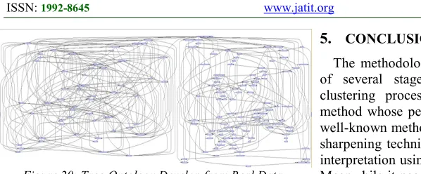
Based on clustering results from table 12 and table 13, is-FADDIS which gives the highest validation value is used into 2-3 KP Real Data R-2. Scatter plots of data clustering using is-FADDIS and sharpening technique with variation of thresholds are shown (figure 19). The third modified data (figure 19c) gives the best separation result (table 14, row 3). This modified data is as an inputted matrix vector using for developing ontology (figure 2). The ontology developed is a tree-ontology (figure 20) which is as a knowledge base for text interpretation.
[image:8.612.313.522.352.446.2]Figure 20: Tree-Ontology Develop from Real Data Sparse R-2
The second step is to correlate inputted text “dua rute baru” into the first sub-ontology with other key phrases related to the inputted text. The correlating result is visuaIized (figure 21). The result is directed relations of parent and child nodes to the inputted text (figure 21, upper) and extended relations (figure 21, below). Another text interpretation result is shown (table 17), which matches with the second sub-Ontology (table 17, row 2). The result of interpretation is visualized as graphs (figure 22).
(a)
(b)
Figure 21: Visualization of Text Interpretation Results with inputted text “dua rute baru”(a) direct relation; (b)
extended relation
All the results of text interpretation are evaluated (table 18). After manual evaluation of visualization of text interpretation, the extracted graph still mixed with other contents or other domains.
5.
CONCLUSIONThe methodology for text interpretation consists of several stages. The contribution in sparse clustering process gives is-FADDIS as a new method whose performance is comparable to other well-known methods, especially if combined with a sharpening technique proposed. Technique for text interpretation using ontology also gives a new way. Meanwhile it needs more improvement in ontology development.
The future works are improvement of ontology development, especially in predicting sub-Ontology and applying the text interpretation into 1-3 KP data.
ACKNOWLEDGMENT
We wish to acknowledge Prof. Boris Mirkin for his contributions to this research. This research was supported partially by Grant from Ministry of Research and Technology of Indonesia.
REFERENCES:
[1] Y. L. N. Zhong, “Effective Pattern Discovery for Text Mining,” IEEE Trans. Knowl. Data Eng., vol. 24, no. 1, pp. 30–44, 2012.
[2] M. Jemni and O. Elghoul, “An Avatar Based Approach for Automatic Interpretation of Text to Sign Language,” Challenges Assist. Technol., vol. 20, no. October, pp. 266–270, 2007.
[3] S. Kurohashi, T. Nakazawa, K. Alexis, and D. Kawahara, “Example-based Machine Translation Pursuing Fully Structural NLP,” English.
[4] C. Su, J. Tian, and Y. Chen, “Latent Semantic Similarity Based Interpretation of Chinese Metaphors,” Eng. Appl. Artif. Intell., vol. 48, pp. 188–203, Feb. 2016.
[5] M. Truyens and P. Van Eecke, “ScienceDirect Legal Aspects of Text Mining,” Comput. Law Secur. Rev., vol. 30, no. 2, pp. 153–170, 2014. [6] Y. Wang, Z. Yu, Y. Jiang, Y. Liu, L. Chen, and Y. Liu, “A Framework and Its Empirical Study of Automatic Diagnosis of Traditional Chinese Medicine Utilizing Raw Free-Text Clinical Records,” J. Biomed. Inform., vol. 45, no. 2, pp. 210–223, 2012.
[image:9.612.89.324.353.633.2][8] F. Rinaldi, K. Kaljurand, and R. Sætre, “Artificial Intelligence in Medicine Terminological Resources for Text Mining over Biomedical Scientific Literature,” Artif. Intell. Med., vol. 52, no. 2, pp. 107–114, 2011.
[9] U. Fayyad, G. Piatetsky-Shapiro, and P. Smyth, “From Data Mining to Knowledge Discovery in Databases,” AI Mag., pp. 37–54, 1996.
[10] D. O. Callaghan, D. Greene, J. Carthy, and P. Cunningham, “Expert Systems with Applications An Analysis of the Coherence of Descriptors in Topic Modeling,” Expert Syst. Appl., vol. 42, no. 13, pp. 5645–5657, 2015. [11] S. Bloehdorn, P. Cimiano, A. Hotho, and S.
Staab, “An Ontology-based Framework for Text Mining,” LDV Forum - Gld. J. Comput. Linguist. Lang. Technol., vol. 20, no. 1, pp. 1– 20, 2004.
[12] H. Wimmer and R. Rada, “Expert Systems with Applications Good versus Bad Knowledge : Ontology Guided Evolutionary Algorithms,” Expert Syst. Appl., vol. 42, no. 21, pp. 8039–8051, 2015.
[13] B. Mirkin, S. Nascimento, and L. M. Pereira, “Cluster-lift Method for Mapping Research Activities over A Concept Tree,” Stud. Comput. Intell., vol. 263, pp. 245–257, 2010. [14] J. Asian, H. E. Williams, and S. M. M.
Tahaghoghi, “Stemming Indonesian,” 2005. [15] I. Veritawati, I. Wasito, and T. Basaruddin,
“Text Preprocessing using Annotated Suffix Tree with Matching Keyphrase,” Int. J. Electr. Comput. Eng., vol. 5, no. 3, 2015. [16] M. Planck and U. Von Luxburg, “A Tutorial
on Spectral Clustering A Tutorial on Spectral Clustering,” Stat. Comput., vol. 17, no. March, pp. 395–416, 2006.
[17] B. Mirkin and S. Nascimento, “Additive Spectral Method for Fuzzy Cluster Analysis of Similarity Data Including Community Structure and Affinity Matrices,” Inf. Sci. (Ny)., vol. 183, no. 1, pp. 16–34, 2012.
[18] F. Shahnaz, M. W. Berry, V. P. Pauca, and R. J. Plemmons, “Document Clustering using Nonnegative Matrix Factorization,” Inf. Process. Manag., vol. 42, no. 2, pp. 373–386, Mar. 2006.
[19] I. S. Dhillon and D. S. Modha, “Concept Decompositions for Large Sparse Text Data using Clustering,” Mach. Learn., vol. 42, no. 1–2, pp. 143–175, 2001.
[20] H. Lu, Z. Fu, and X. Shu, “Non-negative and Sparse Spectral Clustering,” Pattern Recognit., vol. 47, no. 1, pp. 418–426, 2014. [21] R. Studer, R. Benjaminsc, and D. Fensela,
“Knowledge Engineering: Principles and Methods ,” Data Knowl. Eng., vol. 25, no. 1– 2, March, pp. 161–197, 1998.
[22] W. Wong, W. Liu, and M. Bennamoun, “Ontology learning from Text,” ACM Comput. Surv., vol. 44, no. 4, pp. 1–36, 2012. [23] I. Veritawati, I. Wasito, and T. Basaruddin,
“Ontology Model Development Combined with Bayesian Network,” pp. 77–81, 2015.
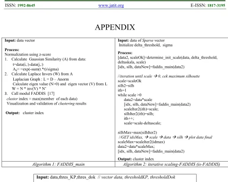
APPENDIX
Input: data vector
Process:
Normalization using z-score
1. Calculate Gaussian Similarity (A) from data: t=data(i,:)-data(j,:)
Aij= =exp(-sum(t.*t)/sigma)
2. Calculate Laplace Invers (W) from A Laplacian Graph : L = D – Anorm
Calculate eigen value (N>0) and eigen vector (V) from L W = N * inv(V) * N’
3. Call modul FADDIS [17]
cluster index = max(member of each data)
Visualization and validation of clustering results
Output: cluster index
Input: data of Sparse vector Initialize delta_threshold, sigma
Process:
[data2, scaleOk]=determine_init_scale(data, delta_threshold, deltaskala, scale)
[idx, silh, dataNew]=faddis_main(data2)
//iteration until scale 0, cek maximum silhoutte
scale=scaleOk silh2=silh ith=1 while scale >0 data2=data*scale
[idx, silh, dataNew]=faddis_main(data2) scaleIter2(ith)=scale;
silhIter2(ith)=silh; ith++;
scale=scale-deltascale;
silhMax=max(silhIter2)
//GET idxMax, scale data silh plot data final
scaleMax=scaleIter2(idmax) data2=data*scaleMax;
[idx, silh, dataNew]=faddis_main(data2)
Output: cluster index
Algorithm 1: FADDIS_main Algorithm 2: iterative scaling-FADDIS (is-FADDIS)
Input: data,thres_KP,thres_dok // vector data, thresholdKP, thresholdDok
process:
data_dense=data; [jKP,jdok]=size(data); // row direction-- document
Add noise (=imaginary value) for document : between (j-thres_dok) and (j+thres_dok) , at data(i,j) put on data_dense
// column direction – key phrase
Add noise (=imaginary value) for key phrase : between (j-thres_KP) and (j+thres_KP) , at data(i,j) put on data_dense
output: data_dense
[image:11.612.81.527.68.425.2]Algorithm 3: Sharpening Technique
Table 3: Validation of Clustering into Data with Normal Distribution
No Method Silhouette Purity Confusion Adj Rand Idx
(1) (2) (3) (4) (5)
1 FADDIS 0.6920 0.9100 0.0900 0.6691
2 NMF 0.2068 0.5900 0.4100 0.0226
3 is-FADDIS 0.7004 0.9300 0.0700 0.7369
4 K-means +norm 0.7004 0.9300 0.0700 0.7369
Table 4: Validation of Clustering with Three Methods into Data Sparse Model-0, Model-3 and Model-6
Data Model
s-Faddis (+scale : 0.015 and 0.051 ) is-Faddis (iterative scale) NMF
Silh PCA
Silh sPCA Purity
Adj. Rand Index
Confu-sion
Silh PCA
Silh sPCA Purity
Adj. Rand Index
Confu-sion
Silh PCA
Silh sPCA Purity
Adj. Rand Index
Confu-sion
(1) (2) (3) (4) (5) (6) (7) (8) (9) (10) (11) (12) (13) (14) (15) (16)
0 0.1008 0.2608 0.6467 0.3876 0.3533 0.2461 0.6594 1 1 0 0.2489 0.6623 1 1 0
3 0.3551 0.5835 0.9333 0.8108 0.0667 0.3540 0.5896 0.9444 0.8386 0.0556 0.3616 0.5988 0.9444 0.8386 0.0556 6 0.1596 0.3462 0.8556 0.6084 0.1444 0.1695 0.3559 0.8556 0.6027 0.1444 0.1906 0.3595 0.9111 0.7453 0.0889
Table 5: Validation of Clustering with Five Methods into Data Sparse Model-15
No Method Silh-PCA Silh- sPCA Purity Confusion Adj Rand Idx
(1) (2) (3) (4) (5) (6)
1 s-Faddis
(+scale : 0.07 ) -0.0396 - 0.6600 0.3400 0.4292
2 is-Faddis 0.0567 - 0.3500 0.6500 0.0461
3 NMF 0.0067 - 0.9667 0.0333 0.9019
4
K-means + without
normalization+ sparse PCA 0.0512 0.2289 0.9600 0.0400 0.8830 K-means+ with
normalization+ PCA 0.0273 0.2510 0.8167 0.1833 0.5288
5 HC 0.4483 - 0.3300 0.6700 -4.4445e-05
Table 6: Validation of Clustering into Model-15using Sharpening Technique Threshold
(KP, dok) – sparse to
dense Data Model
is-Faddis (iterative scale) NMF
Silh PCA
Silh
sPCA Purity
Confu-sion
Adj. Rand Index
Silh PCA
Silh
sPCA Purity
Confu-sion Adj. Rand Index
(1) (2) (3) (4) (5) (6) (7) (8) (9) (10) (11) (12)
0,0 15 0.0567 0.2683 0.3500 0.6500 0.0461 0.0067 0.2559 0.9667 0.0333 0.9019
0,1 15-1 0.0816 0.4707 0.9633 0.0367 0.8937 0.0907 0.5128 0.9833 0.0167 0.9503
1,0 15-2 0.1366 0.6386 0.9867 0.0133 0.9604 0.1380 0.6447 0.9900 0.0100 0.9702
3,0 15-3 0.2944 0.7442 0.9933 0.0067 0.9801 0.2947 0.7446 0.9967 0.0033 0.9900
Table 7: Validation of Clustering into Bupa Dataset
Method Silh Adj RI Purity Confusion
(1) (2) (3) (4) (5)
FADDIS 0.1528 0.0086 0.5652 0.4348 is-FADDIS 0.2315 0.0125 0.5623 0.4377 NMF 0.7280 -0.0124 0.5072 0.4928 K-means 0.8250 -0.0133 0.5304 0.4696 HC 0.8783 -0.0039 0.4319 0.5681
Table 8: Validation of Clustering into Glass Dataset
Method Silh Adj RI Purity Confusion
(1) (2) (3) (4) (5)
FADDIS -0.2492 0.0820 0.2897 0.7103 is-FADDIS 0.2401 0.0415 0.1916 0.8084 NMF 0.1509 0.1673 0.3318 0.6682 Kmeans 0.6105 0.2676 0.4346 0.5654 HC 0.6105 0.2702 0.4579 0.5421
Table 9: Validation of Clustering into CNAE Dataset
method original + sharp , threshold 12-3
Silh Adj RI Purity Confusion Silh Adj RI Purity Confusion
(1) (2) (3) (4) (5) (6) (7) (8) (9)
Table 10: Searching for Optimal Cluster Number using Internal Validation (Silhouette)
Method Model N2 Model-3 Model-6 Model-15 Bupa Glass
(1) (2) (3) (4) (5) (6) (7)
FADDIS o x - x o o
FADDIS p=1 - x x x - -
FADDIS p=2 - x o x - -
FADDIS cos - x - - - -
is-FADDIS o x x o o x
is-FADDIS p=1 - x x x - -
is-FADDIS p-2 - x x x - -
Is-FADDIS cos - o - - - -
is-FADDIS+ - - o o - -
NMF o o o o o x
K-means o x x o o x
HC o x x x o x
Note :
o Fit to cluster number of modeled data x Not Fit to cluster number of modeled data - No experiment
Table 11: Validation of Clustering into Real Data R-1using is-FADDIS and NMF
N o
Real Data
KP number
Doc number
Domain number
is-FADDIS NMF
Silh PCA
Silh
sPCA Purity
Confu-sion
Adj. Rand Index
Silh PCA
Silh
sPCA Purity
Confu-sion
Adj. Rand Index
(1) (2) (3) (4) (5) (6) (7) (8) (9) (10) (11) (12) (13) (14)
1 2-3 KP 729 71 2 0.1739 0.5325 0.3951 0.6049 -0.0706 0.0690 0.1596 0.6680 0.3320 0.0926
2 1-3KP 729+ 460 71 2 0.1318 -0.7409 0.2683 0.7317 -0.0011 0.0437 0.0976 0.5114 0.4886 -1.5158e-04
Table 12: Validation of Clustering into 2-3 KP Real Data R-1using is-FADDIS, NMF and Sharpening Technique
N o
Threshold KP
Threshold
doc Noise
is-Faddis (iterative scale) NMF
Silh PCA
Silh sPCA Purity
Confu-sion
Adj. Rand Index
Silh PCA
Silh
sPCA Purity
Confu-sion
Adj. Rand Index
(1) (2) (3) (4) (5) (6) (7) (8) (9) (10) (11) (12) (13)
1 0 0 - 0.1739 0.5325 0.3951 0.6049 -0.0706 0.0690 0.1596 0.6680 0.3320 0.0926
2 14 2 max. value 0.3714 0.6001 0.7682 0.2318 0.2388 0.3633 0.5845 0.7407 0.2593 0.1927
3 20 2 max. value 0.4446 0.6451 0.7709 0.2291 0.2506 0.4816 0.6373 0.7435 0.2565 0.2023
4 21 2 max. value 0.4622 0.6413 0.7791 0.2209 0.2718 0.4899 0.6416 0.7449 0.2551 0.2055
5 22 2 max. value 0.4738 0.6499 0.7819 0.2181 0.2763 0.5003 0.6502 0.7449 0.2551 0.2046
6 22 2 random(max val) 0.3551 0.6281 0.7737 0.2263 0.2537 0.3357 0.6059 0.7407 0.2593 0.1967
7 22 2 max. value 0.5180 0.6669 0.7833 0.2167 0.2681 0.5003 0.6502 0.7449 0.2551 0.2046
Table 13: Validation of Clustering into 2-3 KP Real Data R-1 using K-means
No. Real Data R-1 Silh-PCA Silh- sPCA Purity Confusion Adj Rand Idx (Ari)
(1) (2) (3) (4) (5) (6)
1 K-means – without
normalization 0.2725 -0.7462 0.7490 0.2510 -0.0053 2 K-means – without
normalization + sharp (Thres 22-2)
0.5312 0.6794 0.7750 0.2552 0.2250
Table 14: Validation of Clustering using is-FADDIS into 2-3 KP Real Data R-2 using is-FADDIS
No. Real Data -2 thKP thdok Silh PCA Silh sPCA Purity Confusion Ari
(1) (2) (3) (4) (6) (7) (8) (9)
[image:13.612.91.469.104.372.2]Table 15: List Inputted Text Query of Inputed Text
(in Indonesian Language) Domain
dua rute baru (two new routes)
badai krisis ekonomi (storm of economic crisis) lion air (lion air)
asia tenggara (southeast asia)
economy
penyelenggaraan piala kemerdekaan (performance the independence trophy) manchester united (manchester united)
pejabat fifa (fifa official)
kualifikasi piala dunia (world cup qualification)
sport
Table 16: Matching Result of Inputted Text “dua rute baru”
Table 17: Matching Result of Inputted Text “asia tenggara”
a
[image:14.612.83.530.310.700.2]b
Figure 22: Text Interpretation of Input : “asia tenggara”
No.SubOn HS Offshoot Gap New Tot-Clust 1. 100.0000 0 98.1818 0 100.0000 2. 0 100.0000 100.0000 0 100.0000
Table 18: Evaluation of Text Interpretation
No inputted Text Interpretation
Evaluation Note
1 dua rute baru A Part Correlation Mix with other topic 2 badai krisis ekonomi No Correlation Mix with other topic 3 lion air No Correlation Mix with other topic 4 asia tenggara A Part Correlation Mix with other topic
5 penyelenggaraan piala