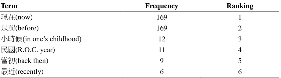
Frequency, Collocation, and Statistical Modeling of Lexical Items:
A Case Study of Temporal Expressions in an Elderly Speaker Corpus
1王聖富 Sheng-Fu Wang
國立臺灣大學語言學研究所
Graduate Institute of Linguistics
National Taiwan University
楊靜琛 Jing-Chen Yang
國立臺灣大學語言學研究所
Graduate Institute of Linguistics
National Taiwan University
張瑜芸 Yu-Yun Chang
國立臺灣大學語言學研究所
Graduate Institute of Linguistics
National Taiwan University
劉郁文 Yu-Wen Liu
國立臺灣師範大學英語學系
Department of English2
National Taiwan Normal University
謝舒凱 Shu-Kai Hsieh
國立臺灣大學語言學研究所
Graduate Institute of Linguistics
National Taiwan University
1 Acknowledgement: Thanks Wang Chun-Chieh, Liu Chun-Jui, Anna Lofstrand, Hsu Chan-Chia, and Liu
Yu-Wen for their involvement in the construction of the corpus and the early development of this paper.
short guideline of transcription standards is provided below.
Conversation samples were manually processed into several IUs. Each IU was labeled
with a number on the left, as shown in example (1).
(1)
34 SM: a 你 看 這 個 做工 的
P. you see this CL. do.work DE 35 ...(1.3) 那 個 有--
that CL. have 36 有夠 重
have.enough heavy
Sometimes speech overlap happened during the conversation. These speech overlaps were
indicated by square brackets, as shown in example (2). In order to indicate on the
transcription when and where utterances overlap, the left brackets of the overlapping
speakers‟ speech are aligned vertically. Double square brackets were used for more overlaps
occurring in a rapid succession within a short stretch of speech, with their left brackets
displaying temporal alignment.
(2)
70 SF: ...都 [送 人家]
all give others
71 SM: [送 人家] [[撫養 la]]
give others to raise P. 72 SF: [[撫養]]
to raise
As bilinguals, the subjects might shift from Mandarin, which dominated the conversation,
to another language. Such utterance of code-switching was enclosed in square brackets and
labeled with L2 as well as the code for the non-Mandarin language. Example (3)
demonstrates the transcription for code-switching, where the language code TSM represents
Taiwanese Southern Min.
(3)
268 SF: [L2 TSM 單輪車 TSM L2]
single wheeler
one token of the symbol @ (see example 4a). Longer laughter was indicated by a single
symbol @ with the duration in the parentheses (see example 4b). Two @ symbols were
placed at each end of an IU to show that the subject spoke while laughing (see example 4c).
(4)
a. 163 F1: @@@@@
b. 200 SM: @(3.3)
c. 828 O: @沒 那麼 嚴重 la@
not that serious P.
The occurrence and duration of a pause in discourse was transcribed. Pauses are
represented by dots: two dots for short pauses that are less than 0.3 seconds, three dots for
medium pauses between 0.3 and 0.6 seconds, and three dots for pauses longer than 0.7
seconds with its duration specified in parentheses. Example (5) below is the instance for
pauses.
(5)
40 SF: ..以前 o..是--
before P. is
41 SF: ...eh ..都 是..父母...(0.9)做 X
P. all is parents do X
Particles were transcribed in phonetic transcription to avoid disagreement on the
employment of homophonic Mandarin characters, as what example (6) shows. Phonetic
transcriptions for the particles included la, hoNh, a, o, le, haNh, hioh, and ma.
(6)
26 SM: hoNh.. a 我們 二十 幾 歲 結婚
P. P. we twenty more age get.married
The recorded utterances were not always audible or clear enough for the transcribers to
identify what was being said. Each syllable of uncertain hearing was labeled with a capital X,
as shown in example (5) above. Last but not least, truncated words or IUs were represented
by double hyphens --, as shown in previous example (1) and (5).
2.3 Annotation
After all recorded samples were transcribed, the transcription would be automatically
agglomerative hierarchical clustering in that a group of entities is first divided into large
groups and then smaller groups are classified. Such a method is useful for finding a few
clusters large in size [22]. We would like to find out whether the terms for “the present” and “the past” can really be grouped into clusters different in temporality. Thus, divisive hierarchical clustering serves our need.
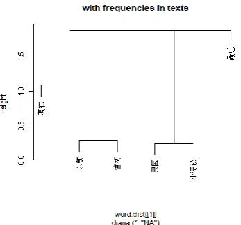
We execute a series of hierarchical clustering with different data input. The first analysis
is run with the frequencies of the temporal terms across different files/texts in our corpus.
Such an input is expected to capture the co-occurrence pattern of these temporal terms
affected by individual speaker‟s style or idiolect, as well as by differences in the conversation topic. The output is presented in Figure 1, where 現在 (now) is separate from以前 (before)
under a major cluster on the left. Also, 最近 (recently) stands independently from any other
expressions, suggesting that temporal terms within a particular time domain are more likely
to occur in the same text, which is really a conversational event in our corpus.
Figure 1. Clustering based on frequencies in texts
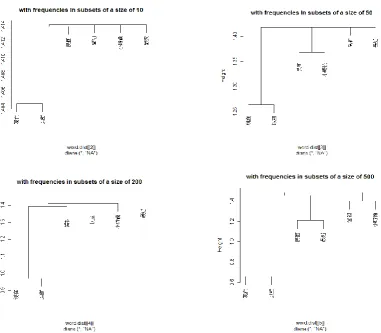
Next, four clustering analyses are made based on the frequency data across subsets of
different sizes. The sizes chosen for producing subsets are 10, 50, 200, and 500 words
respectively. Smaller subsets may reflect linguistic patterns in a few clauses, and larger
subsets may reflect patterns in a larger unit, such as major or minor topics in the flow of conversation. The results are shown in Figure 2. As we can see in the four graphs below, 現 在 (now) and以前 (before) are classified in the same small cluster. It is worth noting that
最近 (recently) is clustered independently with a subset size up to 200, which shows only
Figure 2. Clustering based on frequencies across subsets. Upper left, with subsets of a size of
10 words. Upper right, of 50 words. Lower left, of 200 words. Lower right, of 500 words.
The analyses above are obtained provided with the temporal terms‟ frequencies of
occurrence in different parts of the corpus. In addition to this method, we can also do
clustering analysis according to how these terms collocate with other words in the corpus, on
the premise that collocational patterns should reveal some characteristics of lexical items.
Thus, two more analyses are given based on this assumption. The first analysis is done by using each word type‟s collocational pattern (span = 3) with the six temporal terms as input. The second analysis is achieved through the dependency patterns of sentential particles (i.e.
lah, hoNh, ah, oh, le, haNh, hioh, mah, as described by [23]), taking the temporal terms as its
input. There are two reasons for the inclusion of particle collocation. Firstly, in regard to
methodology, running more than one collocational test allows one to see whether
collocational analyses with different approaches generate similar results. Secondly, sentential particles‟ dependency patterns might help us understand how the “referent” of each temporal expression is conceived and presented in discourse. The outcome is illustrated in Figure 3. Again, 現在 (now) and以前 (before) are clustered closely, showing that their collocational
patterns may be similar, regardless of the actual word types of their collocates. Noteworthily,
Figure 3. Clustering based on association/collocation frequencies. Left, with all word types in
the corpus. Right, with particles.
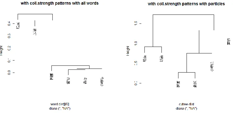
Potentially, there is a problem using raw frequencies in studying collocates. Collocates
with high frequencies might simply be high frequency words rather than being “exclusively close” to the terms of interest. Thus, we bring forth collexeme analysis [24], [25], a statistical method developed for finding “true collocates”, that is, collocates with strong collocational
strength (coll.strength hereafter). The coll.strength of each word type and particle is
calculated and used as input for clustering analysis. The output is shown in Figure 4.
Figure 4. Clustering based on coll.strength patterns. Left, with all word types in the corpus.
Right, with particles.
The next question is: How do we evaluate all these different results? The answer may
a function “cutree” for a simple quantification of different clustering: Each „tree‟ is quantified
in terms of which cluster an item is clustered to. We collect the data for all the trees shown
above and execute clustering as meta-analysis. The outcome is shown in Figure 5.
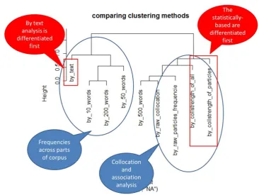
Figure 5. Clustering of various results with different types of input data
An interesting pattern shows up. There are two major clusters. The left one is based on
frequency patterns of temporal terms, and the right one basically contains analyses regarding
how these terms collocate or associate with other words or particles. Despite the curious occurrence of the “by-500-words” analysis in the right major cluster, the result of this meta-analysis seems to be able to characterize the major differences in terms of data input.
More specifically, in the left major cluster, the “by-text” analysis is the first one being singled out. This conforms to our impression that temporal terms are clustered differently, with 現在
(now) and 最近 (recently) placed relatively away from other past-related expressions.
Moreover, in the right major cluster, the analyses with coll.strength are the first ones being
differentiated from the others. Again, it reflects that statistically based analyses produce
different patterns from the ones based on simple frequency values. What can be inferred from
the patterns in Figure 5 is that, first, different types of data input certainly influence the
outcome of clustering analysis, and second, the results of quantitative analysis can also be
evaluated through quantitative analysis, just as how we use hierarchical clustering to analyze
and evaluate results of hierarchical clustering.
[25] S. T. Gries. (2007). Collostructional analysis: Computing the degree of association
between words and words/constructions. Available: