NBER WORKING PAPER SERIES
DSGE MODELS IN A DATA-RICH ENVIRONMENT
Jean Boivin
Marc Giannoni
Working Paper 12772
http://www.nber.org/papers/w12772
NATIONAL BUREAU OF ECONOMIC RESEARCH
1050 Massachusetts Avenue
Cambridge, MA 02138
December 2006
We would like to thank Jesus Fernandez-Villaverde, Alejandro Justiniano, Alexei Onatski, Frank Schorfheide,
Chris Sims, Mark Watson, Michael Woodford, and especially Michael Johannes for helpful discussions.
We also thank Mauro Roca and Huidan Lin for outstanding research assistance. We are grateful to
Frank Smets and Raf Wouters for sharing their data and programs. Any remaining errors are our responsibility.
We would like to thank the National Science Foundation for financial support (SES-0214104, SES-0518770).
Giannoni thanks the Fondation Banque de France and the research department of the Banque de France
for their support and hospitality. The views expressed herein are those of the author(s) and do not necessarily
reflect the views of the National Bureau of Economic Research.
© 2006 by Jean Boivin and Marc Giannoni. All rights reserved. Short sections of text, not to exceed
two paragraphs, may be quoted without explicit permission provided that full credit, including © notice,
is given to the source.
DSGE Models in a Data-Rich Environment
Jean Boivin and Marc Giannoni
NBER Working Paper No. 12772
December 2006
JEL No. C10,C32,C53,E1,E32,E37
ABSTRACT
Standard practice for the estimation of dynamic stochastic general equilibrium (DSGE) models maintains
the assumption that economic variables are properly measured by a single indicator, and that all relevant
information for the estimation is summarized by a small number of data series. However, recent empirical
research on factor models has shown that information contained in large data sets is relevant for the
evolution of important macroeconomic series. This suggests that conventional model estimates and
inference based on estimated DSGE models might be distorted. In this paper, we propose an empirical
framework for the estimation of DSGE models that exploits the relevant information from a data-rich
environment. This framework provides an interpretation of all information contained in a large data
set, and in particular of the latent factors, through the lenses of a DSGE model. The estimation involves
Markov-Chain Monte-Carlo (MCMC) methods. We apply this estimation approach to a state-of-the-art
DSGE monetary model. We find evidence of imperfect measurement of the model's theoretical concepts,
in particular for inflation. We show that exploiting more information is important for accurate estimation
of the model's concepts and shocks, and that it implies different conclusions about key structural parameters
and the sources of economic fluctuations.
Jean Boivin
HEC Montréal
3000, chemin de la Côte-Sainte-Catherine
Montréal (Québec)
Canada H3T 2A7
and NBER
Marc Giannoni
Columbia Business School
3022 Broadway, Uris Hall 824
New York, NY 10027
and NBER
1
Introduction
Recent macroeconomic research has devoted considerable efforts to the development and estimation of dynamic stochastic general equilibrium (DSGE) models that are internally consistent, and based onfirst principles. Some recent micro-founded DSGE models, which involve numerous frictions and various types of shocks, appear to replicate the data in important dimensions (see, e.g., Christiano, Eichenbaum and Evans (2005), Smets and Wouters (2003, 2004)). For instance, Smets and Wouters (2004) report that a DSGE model with a wide range of shocksfits the data well and performs well in terms of out-of-sample forecasts. Motivated by these promising results, such models are now increasingly perceived as a valuable input to policy making.1
In estimating these models, researchers have so far maintained the assumption that all relevant information for the estimation is adequately summarized by a relatively small number (i.e., between three and seven) of data series.2
This is at odds, however, with the fact that central banks and financial market participants monitor and analyze literally hundreds of data series. Moreover, there is growing empirical evidence suggesting that a large set of macroeconomic variables may in fact be crucial to properly capture the economy’s dynamics. In a macroeconomic forecasting context, Stock and Watson (1999, 2002) and Forni, Hallin, Lippi and Reichlin (2000) among others find that factors estimated from large data sets of macroeconomic variables lead to considerable improvements over small scale VAR models.3 Bernanke and Boivin (2003) and Giannone, Reichlin and Sala (2004) show that this large information set appears to matter empirically to properly model monetary policy. Bernanke, Boivin and Eliasz (2005) argue that inference based on small-scale VARs, by omitting relevant
1
For instance, the Bank of Canada is “completing the development of a new projection model– a sticky-price dynamic stochastic general-equilibrium (DSGE) model of the Canadian economy” (see http://www.bankofcanada.ca/en/fellowship/highlights_res.htm). Papers that study optimal policy in estimated medium-sized DSGE models include Juillard, Karam, Laxton and Pesenti (2005), Levin, Onatski, Williams and Williams (2005).
2
The only exception we are aware of is Adolfson, Laséen, Lindé and Villani (2005) which estimates a relatively large model of a small open economy usingfifteen data series. Leeper and Sims (1994) estimated their model with three and ten data series, but report that they were unable to obtain a reasonablefit with ten series.
3Stock and Watson (1999), comparing a wide range of inflation forecasting exercises, found that their best-performing forecast involves a composite index of aggregate activity based on 168 individual activity measures. They argue that the forecasting gains from using this index are economically large and statistically significant over the 1970-1996 sample period. Similar evidence has been found in Forni et al. (2001), Stock and Watson (2002), Bernanke and Boivin (2003) and Boivin and Ng (2003), among others.
information, may be importantly distorted. For instance, they provide evidence in favor of Sims’ (1992) explanation of the “price puzzle,” – i.e., thefinding based on small-scaled VARs that prices tend to increase following a monetary policy tightening – according to which conventional VARs do not account for the information that the central bank has about future inflation. They show that the information from a large set of indicators is indeed important to properly identify the monetary transmission mechanism. These empirical models with large data sets remain however largely non-structural. This limits our ability to determine the source of economicfluctuations, to perform counterfactual experiments, or to analyze optimal policy.
Why would such information be relevant in the context of available DSGE models? If the model of the economy is well specified and all theoretical concepts are directly observed by the agents and the econometrician, there is no scope for using additional data series in the estimation of DSGE models. But if some of the key concepts of the model are imperfectly observed or if the data are informative about some exogenous shocks or other state variables, exploiting the information from additional series could be important.
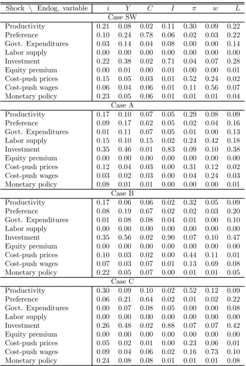
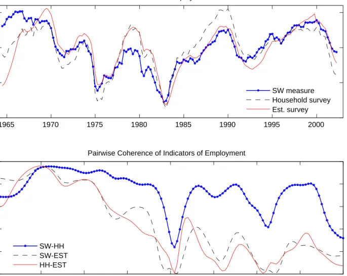
While the assumption that some or all theoretical concepts are observed by the econometrician is routinely made in the estimation of DSGE models, it may not be realistic. The upper panel of Figure 1 plots three detrended quarterly measures of employment (in logs) from 1964 to 2002.4 Figure 2 reports the (de-meaned) quarterly growth rates of popular price measures: the GDP deflator, the personal consumption expenditures (PCE) deflator, and the consumer price index (CPI). While these series display broadly similar patterns, they reveal noticeable differences from one quarter two the next. In fact, as indicated in the lower panels of thefigures, the coherences — i.e., the correlations in the frequency domain — between any two of the series are high at low frequencies, but they are markedly lower, though nonzero, at higher frequencies. If all of thefluctuations in these indicators were attributable to fundamental macroeconomic shocks, one would expect for instance these indicators of inflation to move in sync. However, most high-frequency inflation spikes are not common to all three series considered.
Gaps between several indicators of macroeconomic variables may reflect measurement error.
4
The measure SW is taken from Smets and Wouters (2004), and is described in section 3.2 below. The other two indicators represent employment numbers based respectively on the household and the establishment surveys.
For employment, the systematic discrepancies between its two main measures – one obtained from the establishment survey and the other from the population survey – which have received a lot of attention in the aftermath of the 2001 recession,5 underscore the fact that employment is imperfectly measured.6 Aggregate prices are also notoriously difficult to measure. One of the most commonly used measure, the CPI, has undergone various changes in methodology since the 1996 Boskin commission, to mitigate important shortcomings. But recent research emphasizes that the current CPI might still be subject to important biases, stemming for instance, from the difficulty of measuring quality improvements or properly adjusting for outlet substitution.7 Imperfect measurement may also affect real output, consumption, investment, real wages.
At another level, there may be conceptual differences between the model variables and the data used to measure them. One could of course imagine macroeconomic models to be sufficiently detailed so as to specify a separate role for, e.g., each of the available price indices (such as the GDP deflator, PCE deflator, CPI, core-CPI, and so on). In practice, however, this distinction is rarely made, as there are advantages to analyzing relatively simple models. If follows that researchers often pick a particular price index in a more or less arbitrary way.
Failing to account empirically for the imprecise link between theoretical concepts and observable macroeconomic data can invalidate model estimation and the assessment of whether a particular theoryfits the facts. Following Sargent (1989), this has led some researchers to recognize explicitly the presence of measurement error in their empirical framework.8 However, even when they allow for measurement error, all existing studies that estimate structural models are, to our knowledge, based on at most asingle (and sometimes arbitrary), observable time series corresponding to each variable of the model. That is, whether or not one considers measurement error in the model estimation, it is typically assumed that a small number of data series contain all available information about concepts of the model such as output and inflation.
5See, e.g., Bernanke (2004). 6
The BLS actually reports standard errors for the employment measures based on both surveys in the Employment Report. The non-farm payroll employment number, being based on a larger sample, is statistically more precise. But it is also subject to biases, such as the double-counting of jobs.
7
See Hausman (2003), Hausman and Leibtag (2004) and Bils (2004). 8See, e.g., Altu
˘
g (1989), McGrattan (1994), Anderson, Hansen, McGrattan and Sargent (1996), McGrattan, Rogerson and Wright (1997), Schorfheide (2000), Fernández-Villaverde and Rubio-Ramírez (2004). Another practical motivation for adding measurement error is to avoid the stochastic singularity problem that arises when there are fewer theoretical shocks than observable series.
Once one acknowledges that the data provides only an imperfect indicator of the concept, it is plausible to think that other data series carry useful additional information. Viewed in this light, existing estimations of DSGE models appear to be based implicitly on an arbitrary choice of data. Given each indicator-specific idiosyncrasy, properly exploiting the information from several indica-tors – rather than from a single one – should help to better separate an estimate of the economic concept (such as employment or inflation) from the indicator-specific “measurement error.”9 This should also provide us with a better estimate of the underlying economic shocks.
Moreover, some exogenous shocks or other state variables, that are typically assumed to be completely unobserved by the econometrician, might in fact be partially observed. One example is the productivity shock underlying many DSGE models. In existing estimations, it is treated as completely latent, which amounts to assuming implicitly that no observable measure contains independent information about this shock, beyond the handful of variable used in the estimation. But measures of labor productivity, oil prices, or commodity prices may all be correlated with total factor productivity, and thus serve as noisy indicators containing independent information.10 In principle, since this could be the case for all exogenous shocks, many more indicators could carry important information for the estimation.
In this paper, we propose a general empirical framework to estimate DSGE models that exploits the information from a potentially large panel of data series in a systematic fashion. We relax the common assumption that theoretical concepts are properly measured by a single data series, and instead treat them as unobserved common factors for which observed data series are merely imperfectindicators. We also include information from indicators that potentially have an unknown relationship with the state variables of the model.
The proposed empirical framework has several advantages. First, as a consequence of the factor structure, the latent model concepts and the series-specific component (or “measurement errors”) can be consistently identified from the cross-section of macroeconomic indicators, and not exclusively from the dynamic structure implied by the DSGE model. Consequently, unlike in the
9
In the same spirit, Prescott (1986) used these two indicators to calibrate the labor elasticity of output in his RBC model.
1 0
This is in part the rationale for the inclusion of commodity prices in VARs to “fix” the price puzzle (see Sims (1992)).
standard treatment mentioned above, allowing for measurement error does not necessarily help the model fit the data. Using multiple indicators in the model estimation also allows us to consider a potentially large number of imperfectly measured concepts without restricting the number of structural shocks that can be identified within the model. Rather than taking a stance on whether “measurement errors” or structural shocks should be part of the model, we can remain agnostic and determine empirically their relative importance. A by-product is an empirical assessment of the information content of each indicator.
Second, we can exploit the information from indicators that are not directly and unambiguously linked to a specific concept of the model. If the additional information considered is relevant, it should make our estimation more efficient. This is particularly important to determine more accurately the state of the economy, and helps in forecasting.
Third, our framework can be interpreted as a dynamic factor models à la Stock and Watson (1999, 2002), Forni et al. (2000), Forni, Lippi and Reichlin (2003), Bernanke, Boivin and Eliasz (2005), and Giannone, Reichlin and Sala (2004), in which we impose the full structure of the DSGE model on the transition equation of the latent factors. This has the added benefit of allowing us to provide a very clear economic interpretation of all estimated latent factors: in our setup, these factors correspond to state variables of the model (i.e., predetermined variables or shocks). In contrast, in empirical studies of factor models, the latent factors do not have a clear interpretation, since they are identified only “up to a rotation.” Taken as a whole, the set of the factors obtained in empirical studies spans the space of common components in the data, but each factor does not uniquely characterize a common component. Our framework, in contrast provides an interpretation of all information contained in a large data set through the lenses of a DSGE model.
The estimation involves Markov-Chain Monte-Carlo (MCMC) techniques which deal effectively with the dimensionality problem by working with marginal densities and avoiding gradient methods. Because of the large dimension of models in a data-rich environment, direct estimation by maximum likelihood is usually infeasible in practice. The specific algorithm that we propose extends the standard implementation of Bayesian MCMC methods11 to account for the relationship between a potentially large number of indicators and a relatively small number of model concepts.
1 1
We apply our estimation procedure to a state-of-the-art DSGE model based on microeconomic foundations. The model is taken from Smets and Wouters (2004), which builds on the model of Christiano, Eichenbaum and Evans (2005). One important finding is that by considering infor-mation from a larger data set in our model estiinfor-mation, and by relaxing the link between some indicators and the model’s concepts, we are able to considerably improve the estimates of the model’s latent concepts such as inflation, of state variables and shocks. Our results suggest that the additional information provided by the data-rich environment is highly relevant for the model estimation. Estimates of critical model parameters such as a pseudo-elasticity of intertemporal substitution in consumption, the degree of habit formation, the degree of inflation indexing as well as estimated variances of exogenous shocks differ importantly depending on the assumed link between theory and data. This arises even though the estimated latent variables display patterns generally consistent with the indicators typically used to measure them. The different estimates also imply very different conclusions about the sources of economic fluctuations. As more data series are used in the model estimation, we find that fewer shocks are necessary to explain eco-nomicfluctuations, and that shocks to the efficiency of investment goods become a main source of business cyclefluctuations.
The rest of the paper is structured as follows. Section 2 lays down the formal setup for an arbitrary linear(ized) DSGE model. It explains how we relate the structural model to the large data set, and discusses implications of the setup for a canonical real business cycle (RBC) model. The section then proceeds with a description of the general estimation methodology. Detailed information about the estimation is left in an appendix. Section 3, presents an application of our approach in the context of a state-of-the-art DSGE model, the model of Smets and Wouters (2004), and discusses the estimation results and their implications. Section 4 concludes.
2
Data-Rich Environment
We now present a formal framework that merges a general class of dynamic general equilibrium models with a data-rich empirical model. We then discuss the implications of this framework, both in general terms and in the context of a canonical RBC model.
2.1
General Framework
Let us consider a general linear (or linearized) rational expectations model of the form
AEt ⎡ ⎢ ⎣ zt+1 Zt+1 ⎤ ⎥ ⎦ = B ⎡ ⎢ ⎣ zt Zt ⎤ ⎥ ⎦+Cst (1) st = M st−1+εt (2)
where Et[x]≡E[x|It]denotes the expectation of some variable x conditional on the information
set It available at date t, zt is a vector of non-predetermined endogenous variables, Zt is a
vec-tor containing predetermined endogenous variables or lagged exogenous variables (i.e., satisfying
EtZt+1 = Zt+1), st is a vector of exogenous variables following the process (2), εt is a vector
of mean-zero unforecastable exogenous disturbances (such that Etεt+j = 0 for all j > 0) with a
diagonal variance-covariance matrix Q, and A, B, C and M are conformable matrices of coeffi -cients. Below, we will consider examples of structural dynamic general equilibrium models based on microeconomic foundations that can be cast in the form (1)—(2). Models with additional lags, lagged expectations, or expectations of variables father in the future can be written as in (1) by expanding the vectorszt and Zt appropriately. We assume that the information set in periodt is
It={zτ, Zτ+1, sτ, ετ, forτ ≤t;A, B, C, Q} so that all agents considered in the model are assumed
to know the model, its parameters, and the realizations of all variables determined in the present and past.12 We solve the model using standard numerical techniques,13 and express the solution as
zt = DSt (3)
St = GSt−1+Hεt, (4)
1 2This can be generalized in various ways at the expense of complications for the estimation problem described below. One can for instance assume that some or all of the agents in the model also face imperfect information about the state of the economy, and thus need to solve afiltering problem (see, e.g., Pearlman, Currie, and Levine, 1986, Svensson and Woodford, 2003, 2004) that may or may not be the same as the one of the econometrician described below. The model could still be written in the form (1), except that the vectorszt, Zt, andst would include also estimates on the part of agents of the respective variables. We leave an analysis of imperfect information on the part of economic agents for future work.
where St≡ ⎡ ⎢ ⎣ Zt st ⎤ ⎥ ⎦
is the state vector and the matrices D, G, H are function of the underlying model’s structural parameters.
In many applications, the system (1) contains identities and Zt includes redundant variables
such as lags of variables in zt. We will be interested in a subset Ft of the variables in zt, St (all
known at datet), which refers only to variables characterizing the economy in periodt.The(nF ×1)
vectorFtwill typically include endogenous variables of interest for which indicators are observable.
Specifically, we define Ft≡F ⎡ ⎢ ⎣ zt St ⎤ ⎥ ⎦
whereF is a matrix that selects the appropriate elements of the vector [z0
t, St0]0.Given (3), we can
rewrite the variables of interest as a linear combination of the state vector
Ft=ΦSt, (5) where Φ≡F ⎡ ⎢ ⎣ D I ⎤ ⎥ ⎦ (6)
is entirely determined by the model parameters and the selection of variables inFt.The evolution
of Ft is given by (4)—(6).
In order to estimate the model we consider nX observable macroeconomic variables collected
in a vector Xt. We collect in a nXF ×1 subvector XF,t =
h
x1F,t, ..., xnXFF,t
i0
the indicators of the variables of interestFt= £ f1 t, ..., f nF t ¤0,wheren
XF ≥nF,and assume that the observed indicators
relate to the variables of the model according to
for i = 1, ..nXF, j = 1, ...nF, where for each i, λiF is a coefficient, and eiF,t denotes a
mean-zero indicator-specific component, which may be viewed as representing measurement error or conceptual differences between the theoretical concept ftj and the respective indicator xiF,t. We omit throughout a constant to simplify the notation. We assume that these indicator-specific components are potentially serially correlated, but that they are uncorrelated across indicators. The set of equations (7) can be rewritten in matrix form as
XF,t=ΛFFt+eF,t, (8)
where eF,t is a nXF ×1 vector of mean-zero indicator-specific and potentially serially correlated
components, andΛF is an(nXF ×nF) matrix of coefficients. As each element ofXF,tis supposed
to be an indicator of one of the elements of Ft,each row of the matrix ΛF will have at most one
nonzero element. However, to the extent that each variable inFt can be imperfectly measured by
many indicators, each column ofΛF can have many nonzero elements.
The observation equation (8) is appropriate in the case that several observable indicators relate directly to the same variable of interest, and that each of the indicator-specific components is uncor-related with that of other indicators. For instance, if inflation based on the personal consumption expenditure deflator and the CPI correspond to the same concept of inflation in the model, then one may want to include both indicators inXF,t.However, if these indicators refer actually to different
concepts, then at least one of them should not be included inXF,t.Such an indicator, even though
it does not relate directly to any variable in Ft should still depend on the evolution of the state
vectorSt.
More generally, to the extent that the theoretical model is true, a potentially very large number of indicators observed – e.g., asset prices, commodity prices, monetary aggregates and so on – should depend on the state vector St. Again, it may be useful to consider such indicators in the
estimation, as they may be informative about the state of the model economy. To exploit the information provided by such indicators in the model estimation, we assume that the remaining data series ofXtwhich do not correspond to any particular variable ofFtare collected in anXS×1
vectorXS,t and are related to the state vector according to
XS,t=ΛSSt+eS,t, (9)
where eS,t is anXS ×1 vector of mean-zero components that are not related to the model’s state
vector, and ΛS is an (nXS×nS) matrix of coefficients. Equation (9) allows all indicators not
associated with any particular variable of the model to potentially provide information about the state vector St. We propose to capture the information from the data in XS,t in a non-structural
way, letting the weights in ΛS be determined by the data.
While the weights ΛF relating the variables of interest to their indicators can be interpreted as structural – i.e., policy invariant – the weights ΛS relating the state vector to all other
in-dicators do not need to be so.14 Even though (9) may not be reliable to determine the effects of alternative policies on the variables in XS,t,information about these variables can be very useful
for the estimation of the state vector and model parameters underhistorical policy. Once the state vector and model parameters are correctly estimated – using the information provided by (9) – counterfactual exercises can legitimately be performed for all variablesFt, St, XF,t, without using
(9) any more.
Combining (8)—(9) and using (5), we obtain the observation equation
Xt=ΛSt+et (10) where Xt≡ ⎡ ⎢ ⎣ XF,t XS,t ⎤ ⎥ ⎦, et≡ ⎡ ⎢ ⎣ eF,t eS,t ⎤ ⎥ ⎦, Λ≡ ⎡ ⎢ ⎣ ΛFΦ ΛS ⎤ ⎥ ⎦.
We assume that indicator-specific components eF,t and eS,t are uncorrelated across indicators but 1 4
In fact the weightsΛSmix the weights that the variables inXS,twould attribute to their theoretical counterpart, with the coefficients that relate these theoretical concepts to the state vector St.
serially correlated, so that
eF,t = ΨFeF,t−1+vF,t (11)
eS,t = ΨSeS,t−1+vS,t (12)
where the vectorsvF,tandvS,tare assumed to be normally distributed with mean zero and variance RF andRS,respectively, and where the matricesRF, RSandΨF,ΨSare assumed to be diagonal.15
Our empirical model consists of the transition equation (4) – which is fully determined by the underlying DSGE model –, the selection equation (5), and the observation equation (10)-(12) which relates the model’s theoretical concepts to the data. It contains as an important special case the measurement error framework proposed by Sargent (1989). In the latter framework, each variable inFtcorresponds to a unique observable indicator inXF,t, so that the observation equation
reduces toXt=Ft+et=ΦSt+et.In this casenXS = 0,ΛF =InF,Λ=Φ.A further trivial special
case is one in which model variables are assumed to be directly measured, so that the observation equation reduces toXt=Ft =ΦSt, as in most existing estimations of DSGE models.
The key innovation here is to generalize Sargent (1989)’s framework to the case where the vector of observables,Xt,may be much larger than the vectorFtof variables in the model, i.e. nX >> nF,
and that their exact relationship, summarized byΛ, may be partially unknown. The interpretation is that this large number of macroeconomic variables are noisy indicators of model concepts and thus share some common sources offluctuations. This implies an observation equation with a factor structure similar to the one assumed in the recent non-structural empirical literature which uses a large panel of macroeconomic indicators. However, an important difference with this literature is that, in the present framework, the evolution of the unobserved common components obeys the
1 5We may allow the vectore
S,t to be correlated across indicators, as we may want to include in the vectorXS,t indicators that are driven by some common factors which are not included in the model’s vector of state variables. This could happen for instance if several indicators included inXS,tare part of a same category of indicators, but that their theoretical counterpart is not fullyfleshed out in the model. In this case we would assume that the component of these indicators which is not correlated with the model’s state vector has the following factor structure
eS,t=ΓSe,t+ ˜eS,t
where ˜eS,t is anXS ×1vector of mean-zero indicator-specific (i.e., uncorrelated across indicators) and potentially serially correlated components, and Se,t is a vector of common components in the set of indicatorsXS,t,which are uncorrelated with the model’s state vectorSt.
structure of a DSGE model.
The use of large information sets provides our framework with two important advantages over the existing implementation of DSGE model estimation. First, as the latent variables and the measurement can be identified from the cross-section of macroeconomic indicators, it allows one to identify a much richer pattern of “measurement errors,” even in the presence of many structural shocks. This reduces the risk of biased estimation. Second, it has the potential to yield a more efficient estimation procedure. To illustrate these points, consider the following special case of the framework presented above. Suppose that, according to theory, a variable of interest,ft,satisfies
ft=ρft−1+ηt, (13)
where |ρ| < 1 and the exogenous disturbance ηt is iid.16 Suppose moreover that we observe an indicatorx1tofft.In the case thatx1tconstitutes a perfect measure offt,i.e., that the observation
equation (10) is trivially x1t = ft, the variable of interest ft is known, and the parameter ρ can
easily be estimated by OLS or maximum likelihood. Suppose instead thatx1t is a noisy indicator
of ftand that the observation equation takes the form
x1t=ft+e1t (14)
where e1t is iid.17 In the case that ρ 6= 0, standard techniques such as proposed Sargent (1989)
can be applied to estimatefˆt and disentangle it from the “measurement error,” using the Kalman filter. For this to work, however, we need the stochastic process of ft to be different from the one
that drives the measurement error. In contrast, whenρ= 0,standard techniques cannot be applied to recover the variable of interest ft, asx1t = ηt+e1t is the sum of two variables with the same
stochastic process.18 However, if one or more additional indicators
xit=ft+eit (15)
1 6This is a special case of (4)—(5), wheref
t=Ft=St,εt=ηt,Φ= 1, G=ρandH= 1. 1 7
This is a special case of (10) whereXt=x1t,ΛF = 1,Λ=Φ= 1,andet=e1t. 1 8The likelihood function in this case involves the sum of the variances ofη
t ande1t,so that each variance cannot be identified separately.
for i = 2, .., nX are available, then it is possible to estimate ft even if it is serially uncorrelated.
In fact, ft is a common factor that can be identified through the cross section, on the basis the
observation equations (14)—(15), while the dynamic model (13) is used for identification of the shocks ηt.
More generally, when no more than one indicator is used for any concept of the model – i.e., when nX =nF,as in existing implementations – both the structural shocks and the unobserved
variables have to be identified entirely from the restricted dynamics of the DSGE model, summarized by equations (4)—(5). In that case, having more structural shocks in the model limits the number of independent sources of measurement errors that can be contemplated and it is difficult to formally test whether the resulting model is properly identified or not. Typically, researchers avoid these problems by assuming either no measurement error or few structural shocks. But as argued in the introduction, measurement error or conceptual differences between the measured indicators and the theoretical variables might be quite prevalent, and if so, ignoring them would lead to biased inference.
In contrast, one key feature of factor models with multiple indicators is that the factors can be identified by the cross-section of macroeconomic indicators alone. This implies that in our framework with a factor structure, the large number (nX >> nF) of indicators provides enough
restrictions to identify the latent variables, and the series-specific terms from the observation equa-tion (10). As a result, we can allow for a large amount of measurement errors without restricting in any way the number of structural shocks that can be identified in the model. Rather than taking a stance on which source of variations should be part of the model, we can remain agnostic and determine empirically their importance.
Even when the factors can be identified solely from the model dynamics, as in Sargent (1989), considering the information from the large data set provides another important advantage, namely efficiency of the factor estimation. A key property of factor models is that the variances of the factor estimates are of order1/nX where nX is again the number of indicators inXt.A consistent
estimate of the factors can thus be obtained as nX −→ ∞ (see Forni et al. (2000), and Stock
and Watson (2002), Bai and Ng (2004).) This suggests that exploiting information from a large number of macroeconomic indicators can reduce considerably the uncertainty in the estimated
latent variables, which in turn implies a more efficient estimation of model parameters. Estimation efficiency is then important, in particular for forecasting exercises and policy analysis, as forecasting performance is directly related to precision in model estimates.
It is important to note that by expanding the vector Xt of indicators we are not facilitating
the model’s ability tofit the data. To the contrary, given the factor structure, the more indicators we have in Xt, the more we require the state variables (here kˆt and at) to explain the common
components in the data series, while at the same time satisfying their law of motion given by (20).
2.2
An Illustrative Example: A Simple RBC Model
To clarify how the empirical framework just discussed can be applied to the estimation of a DSGE model, we first discuss a simple example, the canonical RBC model (see, e.g., King, Plosser and Rebelo (1988)). This model allows us also to relate to much of the literature on estimated DSGE models which has often considered variants of the basic RBC model. In section 3, we estimate a more elaborate model that adds numerous frictions to a RBC model of this kind. In the basic RBC model considered here, households maximize their lifetime utility which depends on consumption,
ct,and leisure, 1−lt, E0 ∞ X t=0 βt[log (ct) +vlog (1−lt)], 0< β <1, v >0 (16)
subject to the following restrictions
eatk1t−αlαt = ct+kt+1−(1−δ)kt, 0< α <1, 0< δ <1 (17)
at = ρat−1+vt, 0< ρ <1 (18)
where the exogenous productivity shock at follows a mean-zero AR(1) process. Equation (17)
indicates that output, which is generated using the capital stock kt (chosen at date t−1), hours
worked,lt, and total factor productivity,at,is the sum of private consumption and gross investment.
Solving this household problem yields a set offirst-order necessary conditions which, together with (17) and a transversality condition, characterize the equilibrium evolution of the variables ct, lt,
andkt,for given exogenous disturbances and an initial value of the capital stock. As is well known,
this model admits a unique deterministic steady state in which all endogenous variables remain constant. As a closed-form solution does generally not exist, the model is commonly log-linearized around the steady state. The model’s approximate dynamics around the steady state can be written as ⎡ ⎢ ⎣ ˆ lt ˆ ct ⎤ ⎥ ⎦ = ⎡ ⎢ ⎣ d11 d12 d21 d22 ⎤ ⎥ ⎦ ⎡ ⎢ ⎣ ˆ kt at ⎤ ⎥ ⎦ (19) ⎡ ⎢ ⎣ ˆ kt at ⎤ ⎥ ⎦ = ⎡ ⎢ ⎣ g hρ 0 ρ ⎤ ⎥ ⎦ ⎡ ⎢ ⎣ ˆ kt−1 at−1 ⎤ ⎥ ⎦+ ⎡ ⎢ ⎣ h 1 ⎤ ⎥ ⎦vt (20)
which is of the form (3)—(4) withzt=
h ˆ l,ˆct i0 , St= h ˆ kt, at i0
,and the matricesD, G, H are function only of the model parameters. Here, the circumflex denotes percent deviations from the steady state (e.g.,ˆct≡log (ct/¯c)).
To illustrate the richness of our empirical framework, we consider several variants of the obser-vation equation (10).
No measurement error. A common approach to the estimation of DSGE models is to suppose that we have perfect indicators of the variables of interest. In the case that an indicator Xt = hours1t (e.g., based on the establishment survey) is viewed as measuring perfectly the conceptˆlt,
we may write the selection equation (5) as Ft= ˆlt= [d11, d12]St,so that the observation equation
(10) reduces to
hours1t= ˆlt=d11ˆkt+d12at. (21)
In this case, estimation of the model (19)—(20) with the above observation equation would attribute all variations in the indicatorhours1tto the only source of exogenousfluctuations, the productivity
shock.19
1 9
Given that the RBC model considered here has only one source of exogenousfluctuations, using more than one observable series would result in the model rejection, in the absence of measurement error. In fact, as Ingram et al. (1994) point out, since the number of exogenous disturbances is smaller than the number of endogenous variables, one canfind particular combinations of endogenous variables that are deterministic, so that their variance-covariance matrix is singular. The model is said to be stochastically singular in this case. As this is not true in the data, the model is sure to be rejected.
Standard treatment of measurement error. In the case thathours1tis considered as a noisy
indicator of hours, the observation equation needs to be augmented with a measurement error term,
hours1t= ˆlt+e1t=d11ˆkt+d12at+e1t,
and the standard approach proposed by Sargent (1989) is commonly applied.20 According to this approach, the restrictions of the dynamic model and the Kalman filter are used to estimate the unobserved variables ˆlt,kˆt, at and the measurement error. However, as illustrated in the previous
simple example, such an approach may have trouble disentangling the structural disturbances – the innovations to at – from the measurement error,et,and thus may not be able to identify the
latent variable of interest, ˆlt. Unfortunately, it is difficult to test in practice whether or not the
latent variables and the model parameters are actually identified.
An alternative treatment of noisy indicators: Using multiple indicators of given con-cepts. Once one recognizes that the data often contains noisy indicators of the concepts that one seeks to measure, there is scope for using additional indicators to get better estimates of the model’s parameters and concepts. This can be done generally and systematically in our empirical framework. It suffices to include all relevant indicators in the vectorXt,and to let them be related
to the respective concepts in Ft. For instance, while the establishment survey may provide a good
indicator of the concept of hours worked (hours1t), it is likely to include measurement error that
is uncorrelated with measurement error in the hours as implied by the household survey (hours2t).
Accounting for the information contained in these two measured series may thus help us get a better estimate of the concept of hours worked and the model parameters.21 The observation (10) then takes the form
⎡ ⎢ ⎣ hours1t hours2t ⎤ ⎥ ⎦= ⎡ ⎢ ⎣ 1 λ ⎤ ⎥ ⎦ˆlt+et= ⎡ ⎢ ⎣ d11 d12 λd11 λd12 ⎤ ⎥ ⎦ ⎡ ⎢ ⎣ ˆ kt at ⎤ ⎥ ⎦+ ⎡ ⎢ ⎣ e1t e2t ⎤ ⎥ ⎦.
2 0See, e.g., Altu ˘
g (1989), McGrattan (1994), Hall (1996), McGrattan, Rogerson and Wright (1997), and Ireland (2004).
2 1In the same spirit, Prescott (1986) used these two indicators of hours worked to calibrate the labor elasticity of output in his RBC model.
All indicators of hours are thus assumed to have one common factor,ˆlt,on which they “load” with
a particular weight. We typically normalize one of the loading coefficients to 1 so as to normalize the scale of the fluctuations in the latent variableˆlt to be of the same order of magnitude as the
respective indicator, but leave the other loading coefficient free to be estimated, in case the fl uctu-ations in the second indicator are of a different magnitude. By exploiting both the cross-sectional and the time series characteristics of the data, and noting that the latent variables are assumed to generate the common variation in both indicators, while the “measurement error” is specific to each series, we can more easily estimate the latent variables here than in the standard treatment of measurement error. The observation equation mentioned here only exploits information about employment, but one could easily augment it with indicators of other variables.
Using information to estimate the state vector through an unknown link. So far, we have assumed thatΛSis a zero matrix. We have thus implicitly assumed, as do current estimations of DSGE models, that the data series in XS,t, which do not measure any specific variable of the
vectorFt – here, hours worked – do not contain any additional information about the remaining
latent variables.22 However, if the theoretical model is true, all economic data series should at
least partly determined by the state vector. Data on stock prices, commodity prices, oil prices, monetary aggregates and so on could thus be informative about the current state of the economy, even though the model does not explicitly specify model such concepts. Exploiting their information content should result in a more efficient estimation. In our simple example, if oil prices (P oilt) are
systematically related to the state vector of the model economy, we can augment our observation equation as follows ⎡ ⎢ ⎢ ⎢ ⎢ ⎣ hours1t hours2t P oilt ⎤ ⎥ ⎥ ⎥ ⎥ ⎦= ⎡ ⎢ ⎢ ⎢ ⎢ ⎣ d11 d12 λd11 λd12 λS1 λS2 ⎤ ⎥ ⎥ ⎥ ⎥ ⎦ ⎡ ⎢ ⎣ ˆ kt at ⎤ ⎥ ⎦+ ⎡ ⎢ ⎢ ⎢ ⎢ ⎣ e1t e2t e3t ⎤ ⎥ ⎥ ⎥ ⎥ ⎦
where the new parameters λS1 and λS2 are to be estimated.
2 2Several studies, including Christiano (1988), Altu ˘
g (1989) and McGrattan (1994), assume that the capital stock is observed, so that it would be in Ft.They however assume that other variables are latent. McGrattan (1994), for instance, using a more elaborate variant of the RBC model presented here assumes that output, investment, government purchases, hours of work, the capital stock and various tax rates are observed, while housing starts and past hours (weighted) are assumed to be latent.
2.3
Estimation Procedure
We now discuss the general procedure for the estimation of the parameters and the latent variables (in zt, Zt, st) of the structural model (1). This model results in an equilibrium characterized by
(3)—(5). We suppose that the observation equation takes the form (10), where we allow Xt to
potentially contain a rich set of macroeconomic indicators, and where Λ involves possibly few a priori restrictions. Doing so obviously comes at a cost. The high-dimensionality of the problem and the presence of unobserved variables considerably increase the computational burden of the estimation. In particular, methods that rely on explicitly maximizing the likelihood function or the posterior distribution appear impractical (see Bernanke, Boivin and Eliasz (2005)).
To circumvent this problem, we consider a variant of a Markov Chain Monte Carlo (MCMC) algorithm.23 There are two key general features of these simulation-based techniques that help
us in the present context. First, rather than working with the likelihood or posterior directly, these methods approximate the likelihood with empirical densities, thus avoiding gradient methods. Second, by exploiting the Clifford-Hammersley theorem, these methods sample iteratively from a complete set of conditional densities, rather than from the joint density of the parameters and the latent variables. This is particularly useful when the likelihood is not known in closed form, as it is the case in our application. Moreover, by judiciously choosing the break up of the joint likelihood or posterior distribution into the set of conditional densities, the algorithm deals effectively with the high dimensionality of the estimation problem.
Like in existing Bayesian implementations of the MCMC algorithm, the structural parameters of equation (1) are drawn using a Metropolis step, since their distribution conditional on the unobservable state variables and the parameters of equations (3)—(4) are not known in closed form. The unobservable states are drawn using Carter and Kohn (1994) forward-backward algorithm. The remaining parameters are drawn directly from their known conditional distributions. The precise description of the algorithm is provided in Appendix A.
2 3
See Johannes and Polson (2004) for a survey of these methods and Geweke (1999). Recent applications to the estimation of DSGE models include DeJong, Ingram and Whiteman (2000), Schorfheide (2000), Otrok (2001), Smets and Wouters (2003, 2004), Fernández-Villaverde and Rubio-Ramírez (2004), Justiniano and Preston (2004), and Justiniano and Primiceri (2006).
3
Application: Estimating a DSGE Model
3.1
Model
We now apply the data-rich environment just described to a state-of-the-art DSGE model based on microeconomic foundations. The model that we consider is taken from Smets and Wouters (2004). It builds on the canonical RBC model presented in the previous section, as well as Rotemberg and Woodford (1997), Christiano, Eichenbaum and Evans (2005) and others, by adding various frictions and allowing for nine different types of exogenous disturbances. The canonical RBC model can be viewed as a special case of the Smets and Wouters (2004) model in the absence of frictions and of shocks, except for the total factor productivity shock. The Smets and Wouters model has received much attention recently, in part because of its success infitting actual data, both in the U.S. and in the Euro area (see Smets and Wouters, 2003, 2004). As Smets and Wouters (2004) report, this micro-based model performs also surprisingly well in terms of out-of-sample predictions, in some cases outperforming standard VAR and Bayesian VAR models.
A derivation of the non-linear model from first principles can be found in Smets and Wouters (2004). Here, we merely summarize the important log-linearized equilibrium conditions of the model. The model involves optimizing households that consume goods and services, supply spe-cialized labor on a monopolistically competitive labor market, rent capital services to firms, and decide how much capital to accumulate. Firms choose the desired level of labor and capital inputs, and supply differentiated products on a monopolistically competitive goods market. Prices and wages are optimized at random intervals as in the Calvo (1983) model. When they are not re-optimized, prices and wages are partially indexed to past inflation rates. While Smets and Wouters (2004) assume an exogenously moving inflation target, so as to allow in a crude way for changes in the monetary policy rule and in average inflation over the 1957 - 2002 period, we do not consider such time-varying target, as we estimate the model using data from 1982 to 2002.
More precisely, the model assumes that there exists a continuum of households who derive utility from consumption and leisure. The utility function is non separable in consumption and leisure as in King, Plosser and Rebelo (1988) and Basu and Kimball (2000), to allow for a steady state growth path driven by labor-augmenting technological progress, and involves consumption in
excess of an external, time-varying habit stock. While households may be heterogenous regarding their wage profile and hours worked, there exists a complete set of state-contingent securities which allows households to pool their risks, so that they all make the same consumption and investment decisions. The Euler equation for optimal consumption decisions log-linearized around the deterministic steady state with constant growth and zero inflation is given by
Ct = h 1 +hCt−1+ 1 1 +hEtCt+1+ σc−1 σc(1 +λw) (1 +h) (Lt−EtLt+1) −(1 +(1−hh))σ c (it−Etπt+1) +εbt (22)
whereCtandLtrepresent percent deviations of consumption and hours worked from their respective
steady state,it denotes deviations of the quarterly nominal interest rate from its steady-state level,
and πt is quarterly inflation. The parameter h∈(0,1)measures the degree of habit formation and σc > 0 indicates the curvature of the utility function with respect to consumption, and (1 +λw)
is the steady-state markup of the real wage due to market power on the labor market. In the absence of habit formation, (22) states that consumption depends negatively on the ex-ante real interest rate with a coefficient σ−c1 (corresponding to the elasticity of intertemporal substitution) and positively on expected future consumption. When h >0, current consumption is also higher the higher past consumption. Whenσc>1,hours worked and consumption are complementary.24
Finally the exogenous disturbance εbt is a preference shocks that affects the entire utility function and that is assumed to follow and AR(1) process with degree of serial correlation ρb.
On the labor market, households are assumed to re-optimize their wages given the demand for their labor services, with a probability 1−ξw. When choosing their optimal wage they take into account the probability that wages will not be re-optimized for some periods. Whenever they cannot re-optimize their wages, they index them to lagged inflation with a degree of indexationγw ∈(0,1).
Optimal wage setting by households results in the following aggregate linearized equation for the
real wage wt = β 1 +βEtwt+1+ 1 1 +βwt−1+ β 1 +βEtπt+1− 1 +βγw 1 +β πt+ γw 1 +βπt−1 −(1 +λβw) ((1λ−βξw) (1−ξw) w+ (1 +λw)σL)ξw ∙ wt−σLLt− σc 1−h(Ct−hCt−1) +ε L t ¸ +ηwt (23)
where wt is the percent deviation of the real wage from the steady state path, εLt is a shock to
the disutility of labor, which follows an AR(1) process with degree of serial correlation ρL,and ηwt
is an iid shock to the wage mark-up. The parameter β ∈ (0,1) is the subjective discount factor,
σ−L1 >0 is the elasticity of work effort with respect to the real wage. The term in square brackets corresponds to the gap between the actual real wage and the real wage that would prevail in the case offlexible prices andflexible wages. A positive gap tends to reduce the actual real wage, and the effect is stronger the smaller the degree of wage rigidity, ξw, the lower demand elasticity for specialized labor, (1 +λw)/λw, and the higher the elasticity of labor supply with respect to the
real wage, σ−L1.
Households choose the capital stock which they rent to firms. To increase the supply of capital services, they can either invest in future capital, or increase the utilization rate of installed capital. Investment in capital takes one period to be installed and involves adjustment costs which assumed to be function of the change in investment, as in Christiano, Eichenbaum and Evans (2005). As in Greenwood, Hercowitz and Krusell (1998) and Fisher (2002), the relative efficiency of investment goods is also assumed to be affected by an exogenous shockεIt which follows an AR(1) process with degree of serial correlationρI.The log-linearized Euler equation for optimal investment is given by
It= 1 1 +βIt−1+ β 1 +βEtIt+1+ 1/ϕ 1 +β ¡ Qt+εIt ¢ (24)
where It denotes real investment and Q is the real value of capital, in percent deviations from
steady state, and ϕis a measure of adjustment costs. The real value of capital follows in turn
Qt=−(it−Etπt+1) + 1−τ 1−τ+ ¯rkEtQt+1+ ¯ rk 1−τ+ ¯rkEtr k t+1+η Q t , (25)
on the expected future real value of capital and the expected future rental rate of capital rtk.
The mean rental rate of capital ¯rk and the depreciation rate of capital, τ , are assumed to satisfy
β = 1/¡1−τ+ ¯rk¢.The exogenous shockηQt ,assumed to be iid, is meant as a shortcut for changes in the externalfinance premium. The capital accumulation equation then involves both theflow of investment, and its relative efficiency
Kt= (1−τ)Kt−1+τ It−1+τ εIt−1. (26)
There is a continuum of firms that hire aggregates of labor and capital (adjusted for effective utilization) as inputs, combine them using a Cobb-Douglas production function with constant re-turns to scale, and a capital shareα∈ (0,1),and supply a differentiated intermediate good on a monopolistically competitive market. In producing their goods, all intermediate firms face a fix cost and a common stationary technology shock,εat,assumed to be AR(1) with degree of serial cor-relationρa,and labor augmenting technological progress growing at a constant rate. Intermediate goods are then aggregated into a singlefinal good used for consumption or investment. Minimizing thefirms’ cost of production results in the linearized demand for labor
Lt=−wt+ (1 +ψ)rtk+Kt−1. (27)
This implies that for a given stock of capital, the labor demand depends negatively on the real wage and positively on the capital stock and the rental rate of capital, where ψ >0 is the inverse of the elasticity of the capital utilization cost function.
Similarly to households on the labor market, firms are assumed to re-optimize their prices given the demand for their goods, with a probability1−ξp.When they cannot re-optimize their prices, they index them to lagged inflation with a degree of indexationγp ∈(0,1). Optimal price setting by firms results in the following aggregate linearized equation for inflation
πt= β 1 +βγpEtπt+1+ γp 1 +βγpπt−1+ ¡ 1−βξp¢ ¡1−ξp¢ ¡ 1 +βγp¢ξp h αrkt + (1−α)wt−εat i +ηpt. (28)
inflation and on the marginal cost, here represented by the expression in brackets. The marginal cost depends in turn on the real rental rate of capital, the real wage, the productivity shock. To the extent that prices are indexed, current inflation is also affected by lagged inflation. The exogenous shockηpt is assumed to be iid and refers to exogenous fluctuations in the price mark-up.
The linearized goods market equilibrium condition can then be written as
Yt = (1−τ ky−gy)Ct+εtG+τ kyIt+ ¯rkkyψrkt (29) = φ h εat +αKt−1+αψrkt + (1−α)Lt i (30)
where ky is the steady-state capital-output ratio, gy is the steady-state government
spending-output ratio, and φis one plus the share offixed cost in production, andψ is again the inverse of the elasticity of the capital utilization cost function. Government spending (in percent deviation from steady state, timesgy),εGt ,is assumed to evolve exogenously and to follow and AR(1) process
with serial correlation ρG. While the first equation corresponds to the aggregate demand side for output, the second equation results from aggregate production.25
The model is closed with a specification of an empirical monetary policy reaction function. Here, we assume that monetary policy follows the generalized Taylor rule
it= (1−ρ) [rπ0πt+rπ1πt−1+ry0Yt+ry1Yt−1] +ρit−1+ηit (31)
where ηit is an iid monetary policy shock. The specification considered here differs slightly from the one in Smets and Wouters (2004): while we suppose that the central bank responds to actual outputfluctuations (in deviations from the steady-state trend), Smets and Wouters (2004) assume that the central bank responds to deviations of output from the output that would obtain in the case offlexible prices andflexible wages.26
The model is thus summarized by the ten equations (22)—(31). It involves ten endogenous
2 5In thefirst equation, we corrected the equilibrium condition indicated in Smets and Wouters (2004), adding the termr¯kkyψrtkas in Onatski and Williams (2004).
2 6
Their “output gap” may be considered more appropriate as it corresponds to the welfare relevant output gap, in the context of this model. It however differs substantially from empirical measures of “output gap” or the CBO’s measure. In addition, their measure of output gap requires the specification of a significantly larger model, as the flexible-price, flexible-wage counterpart to the equations mentioned above need to be adjoined to the model, to determine theflexible-price,flexible-wage level of output.
variables Yt, Ct, It, Lt, Kt, Qt, rkt, πt, wt, it, and nine exogenous disturbances, five of them
auto-correlated (εat, εbt, εGt , εLt, εtI) and four iid (ηQt , ηwt, ηpt, ηit). The system can then be written as in (1), and can be solved using numerical techniques to obtain a solution of the form (3)—(4), where
zt is a vector of endogenous non-predetermined variables, Zt contains predetermined endogenous
variables as well as lagged exogenous variables, andεtis the vector of innovations to the 10 shocks.
In the estimation, we will use indicators of the following vector of variables of interest
Ft= [it, Yt, Ct, It, πt, wt, Lt]0.
This vector is related to the state vector
St= h it−1, Yt−1, Ct−1, It−1, πt−1, wt−1, Kt−1, εat, εtb, εGt , εLt, εIt, η Q t , η p t, ηwt, ηit, εIt−1 i0
through (5)-(6). This state vector follows a law of motion of the form (4).
3.2
Implementation of the Estimation
3.2.1 Data
Smets and Wouters (2004) estimate their model using quarterly U.S. data starting in 1957. However, given the evidence provided about the instability of interest rate rules of the form (31), especially around the end of the 1970’s and early 1980’s (see, e.g., Clarida, Galí and Gertler (2000), Boivin (2005), Boivin and Giannoni (2006)), we estimate the model starting in 1982:1 and ending in 2002:3. Our large data set contains 91 macroeconomic indicators.27 Details are provided in Appendix B.
Seven data series, included in a vectorX1,t are however worth emphasizing as they are used to
normalize the seven concepts of the model included in the vector Ft. They are the series used by
Smets and Wouters (2004) for the estimation of their model. For each of these series, we normalize the corresponding weights in Λ to 1. Output (Yt) is normalized to real GDP. Consumption (Ct)
and investment (It) are normalized respectively to personal consumption expenditures and fixed 2 7
These are indicators of real output, compensation and wages, employment and hours, consumption, investment, interest rates, money, credit, prices, and some miscellaneous indicators.
private domestic investment.28 The labor input (Lt) corresponds to hours worked per person.29
All preceding series are expressed in per capita terms by dividing with the population over the age of 16. The real wage (wt) is normalized with the hourly compensation for the nonfarm business
sector, divided by the GDP deflator. We express all these series in natural logs and remove a linear trend, so that they are expressed in percentage deviations from the trend, consistently with the model concepts. Inflation (πt) is measured as the quarterly percentage change in the GDP deflator.
The nominal interest rate (it) is the Federal funds rate. Both inflation and the interest rate are
demeaned, to be consistent with the model’s concepts.
Smets and Wouters (2004) assume that in steady-state, the above series are all growing at the rate of labor-augmenting technological progress, and they estimate their model imposing the common trend. This assumption is unfortunately rejected by the data (see Del Negro, Schorfheide, Smets and Wouters, 2004). To circumvent this issue, we detrend all series before the model es-timation, so that the model parameters are estimated on the basis of deviations from the steady state.
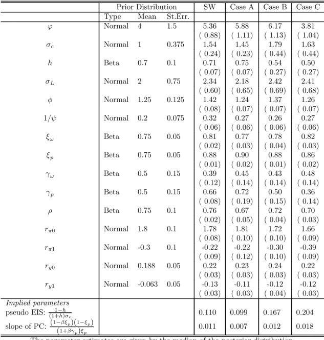
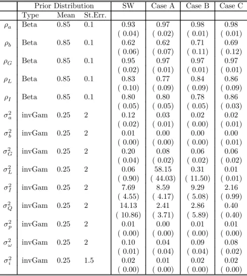
3.2.2 Prior distributions of the parameters
As mentioned above, we estimate the DSGE model using Bayesian MCMC methods. We assume the same prior distributions as in Smets and Wouters (2004). These priors are summarized in Table 1 and are discussed in more details in Smets and Wouters (2004). Six of the structural parameters are calibrated, as they are difficult to estimate from percent deviations from the steady state. The discount rate β is set at 0.99, the quarterly depreciation rate τ is set at 0.025, the share of consumption(1−τ ky−gy) and investment (τ ky) are set at 0.65 and 0.17, which implicitly define gy andky. The capital-income share in the production function,αis set at 0.24. The parameterλw
is fixed at 0.5. One difference with respect to Smets and Wouters (2004) involves the parameters of the policy rule which we assume takes the form of a generalized Taylor rule. The (long-run) response of the (annualized) federal funds rate to (annualized) inflation is assumed to be normally
2 8The nominal series for consumption and investment are deflated with the GDP deflator, as in Altig, Christiano, Eichenbaum and Lindé (2003), and Smets and Wouters (2004).
2 9As in Smets and Wouters (2004), average hours of the nonfarm business sector are multiplied with the civilian employment to account for the limited coverage of the nonfarm business sector, compared to GDP.
distributed with a mean of 1.5 and a variance of 0.5, and the response to detrended output is assumed to have a mean of 0.5 and variance of 0.2. The degree of inertia in monetary policy, or the response to the lagged interest rate is beta distributed with a mean of 0.75 a standard deviation of 1. Finally, fairly loose priors are assumed on the degree of measurement error. More details are provided in Appendix A.
3.2.3 Alternative specification of the observation equation: Four cases
We now proceed with the model estimation. To assess the importance of measurement error and of additional information, we consider four cases, each involving different restrictions on the observation equation (10), i.e., on the link between the model concepts and the data.
• Our first case, denotedCase SW corresponds to the standard estimation with a small set of data series, assuming that there is no measurement error. This case effectively attempts to replicate the results of Smets and Wouters (2004).30 The seven key model variables included in Ft are assumed to be perfectly observed, and only the associated time series mentioned
above – included inX1,t – are used in the estimation. In terms of our general notation, the
observation equation (10) reduces toX1,t=Ft=ΦSt.
As argued above, it is plausible that the indicators in X1,t measure only imperfectly the model
concepts. If this is true, the estimates of the model parameters and of the shocks should be distorted. We thus consider three different cases in which we allow the indicators collected inX1,tto include a
series-specific component (or measurement error) that is unrelated to the actual economic concept,
Ft. We however maintain throughout the assumption that the nominal interest rate is perfectly
observed.
• In our benchmark case with imperfect measurement, denoted Case A, we reestimate the model with the same seven data series but allowing for “measurement error” (except for the nominal interest rate). The observation equation is thus X1,t =Ft+e1,t=ΦSt+e1,t where 3 0As mentioned above, our estimation differs slighlty from the baseline case of Smets and Wouters (2004) for the following reasons: We consider a slightly different policy rule, we detrend the data before estimating the model parameters instead of estimating a common trend (the growth rate of technology) with the rest of the model, we assume that the inflation target isfixed, and we use a shorter sample.
the first element of e1,t is set equal to zero. The setup corresponds to the one in Sargent
(1989), where the restrictions of the dynamic model are used to estimate the latent variables inFt.
As discussed in Section 2, Case A is likely to be affected by identification problems due to the difficulty in disentangling the structural disturbances εt from the measurement errors e1,t, in
the face of a large number of shocks and measurement errors. Such problems can be addressed by considering a larger data set which can more easily identify the latent variables of interest by separating the series-specific components from the common factors,Ft. In the next cases, we thus
maintain the observation equationX1,t =Ft+e1,t, but append to it another observation equation
including additional indicators.
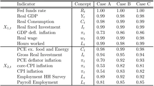
• InCase B, we add seven new indicators collected in a vectorX2,t,which have a known link to
the variables in Ft.These additional indicators are selected on the grounds that they cannot
be a priori rejected as indicators of the variables of interest.31 The observation equation for
this second set of indicators is of the form X2,t = Λ2Ft+e2,t, where each element of e2,t is
allowed to follow an AR(1) process. The matrix Λ2,which we estimate, is restricted to have as many nonzero elements per column as there are new indicators inX2,t of the corresponding
variable inFt. It has however no more than one nonzero element per row as each indicator is
assumed to load on only one variable.
• Ourfinal case,Case C, exploits the information from our entire data set in aflexible way. The fourteen primary indicators contained inX1,t andX2,t remain linked to the model’s concepts
as in case B, but we augment the vector X2,t with eight additional indicators of inflation
which we link to the variableπt, as documented in Appendix B. In addition, we introduce in X3,t information from all other indicators and assume thatX3,t is related to the state vector St in a nonstructural way, according to the observation equation X3,t = ΛSSt+eS,t. The
elements of X3,t are the 25 principal components of all remaining data series listed in our 3 1
For consumption, the new indicator is real personal consumption expenditures excluding food and energy, for investment we add real gross private domestic investment, for inflation we add the indicators based on the deflator for personal consumption expenditures, the CPI, and the CPI less food and energy. For employment, we add the number of employees in the nonfarm business sector, as based on the establishment survey, and the number of workers as based on the household survey.
Appendix B. Each element of eS,t is assumed to follow an AR(1) process, and the loading
matrixΛS is left unrestricted and is estimated.
The motivation for this last specification comes from the fact that if the theoretical model is true, the data series in X3,t should be related at least in part to the state vector. These indicators
are publicly available. They are thus arguably part of the information set according to which economic agents in the DSGE model base their decisions. If these indicators contain information about the state of the economy that is not included inX1,tandX2,t,then exploiting this information
should help us obtain even more accurate estimates of the state of the economy and of the model parameters.
In case A, we assume the “measurement error,” e1,t,to be serially uncorrelated, as this
restric-tions is necessary to identify the model parameters. Whenever we let e1,t to be serially correlated
in this case, we obtain estimated model parameters that are perfectly aligned with the prior distri-butions, suggesting that the data is uninformative, i.e., that the parameters are unidentified. As conjectured in Section 2, this highlights the fact that for models with a large number of structural shocks, and using a small set of observable variables, the extent to which measurement error can be allowed is severely limited using standard techniques. For comparison with this standard approach (case A), we assume that the measurement error in the primary indicators is also iid in cases B and C (even though we can relax this assumption in these cases, and still be able to identify the model parameters). We however allow the measurement errors of the secondary indicators (e2,t or eS,t) to be serially correlated. By restricting the indicator-specific error terms to be iid, we may
understate the magnitude of the series-specific component in the primary indicators X1,t. This
guarantees that the departures from the standard setups (cases SW and A) are relatively small. Nonetheless, as we show below, even for such small departures there are important benefits from exploiting information from a richer data set.
3.3
Empirical Results
We now describe the empirical results. Wefirst provide evidence indicating that some of the seven primary indicators contain a nontrivial amount of series-specific idiosyncrasies, so that estimation
allowing for it should be warranted. We next argue that estimating the model with a richer data sets provides a number of benefits among which a more accurate estimate of the state of the model economy.
3.3.1 Evidence of indicator-specific component (or “measurement error”)
According to the observation equation (10), each of the indicators can be decomposed into a “macro-economic component,”ΛSt,which is informative about the latent macroeconomic concepts, and an
indicator-specific component (or “measurement error”), et.
Table 2 reports correlations between the indicators collected inX1,t, X2,t,and the corresponding
model concept. Looking at the seven primary indicators, X1,t, there is evidence of substantial
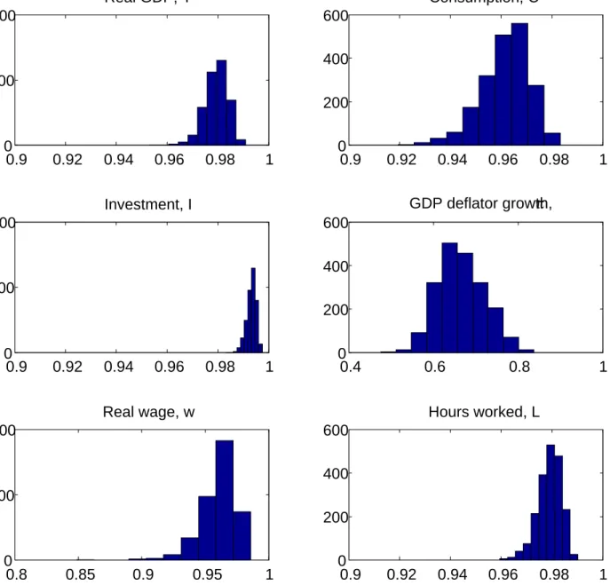
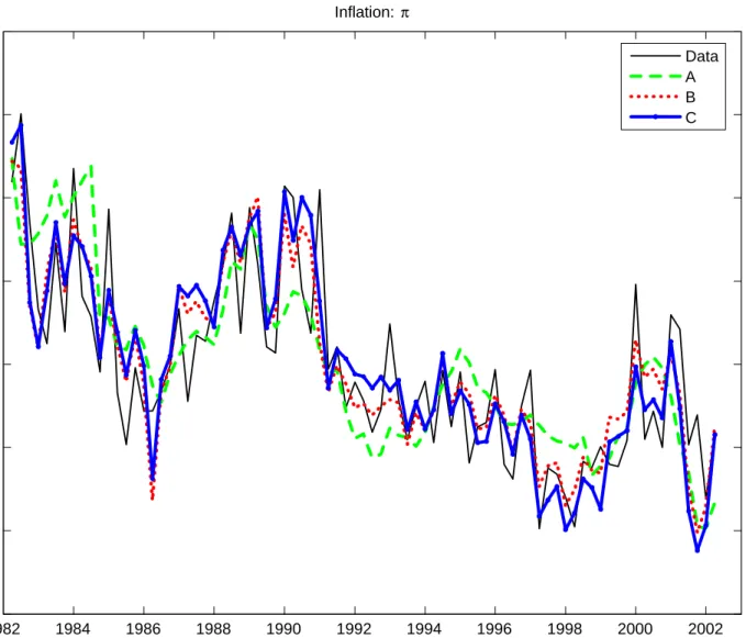
“measurement error” for the indicator of inflation. The correlation between the growth rate of the GDP deflator and the estimate of inflation ranges between 0.73 and 0.86 depending on the number of indicators used in the model estimation. For other indicators in X1,t, the extent of
“measurement error” appears small. Figure 3 plots the posterior distribution of these correlations, in case A. Similar figures – not reported – are obtained for cases B and C. Clearly there is considerable “measurement error” in the growth rate of the GDP deflator. But the figure shows also that at any confidence level, the correlations are slightly lower than 1 for all indicators except for the Federal funds rate which is assumed to be perfectly correlated withit.
The lower panel of Table 2 suggests that the additional indicators X2t provide relevant
infor-mation for the model concepts: while their correlations with the corresponding model variables are relatively low in case A, they increase when they are used in the estimation (cases B and C). Interestingly, the PCE deflator provides a better indicator of the concept of inflation than the GDP deflator, when judged on the basis of their correlation with the estimated concept of inflation, in cases B and C.
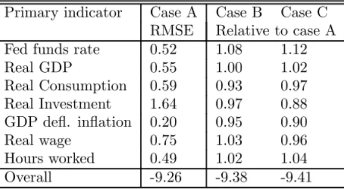
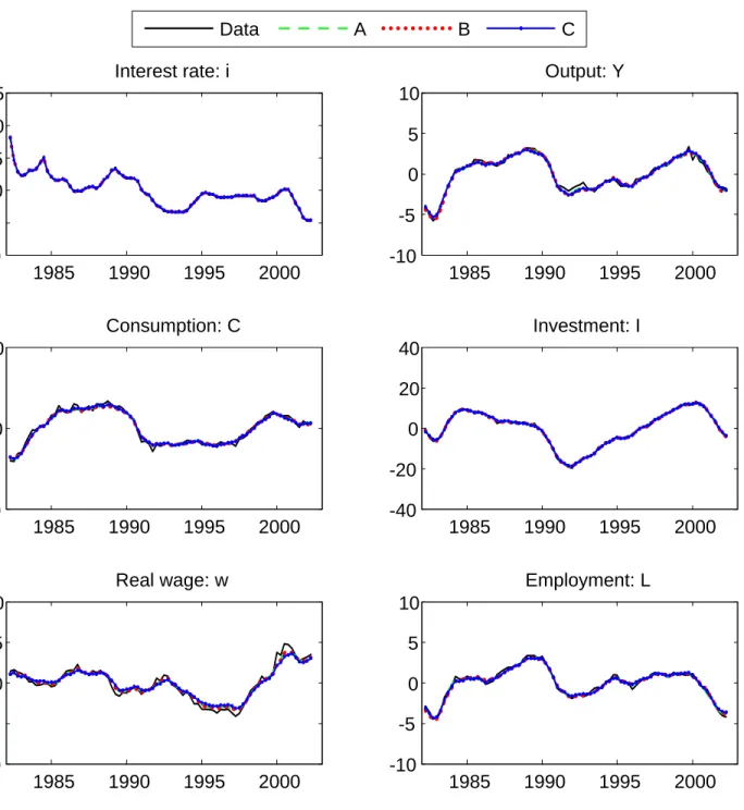
Figures 4 and 5 report the estimated time series of the seven main endogenous variables for each of the cases SW, A, B and C. In case SW, the estimated series correspond to the primary indicators which are represented with solid lines. In the other cases, the model’s concepts except for the short-term interest rate are estimated latent variables. Overall, these plots confirm the results found in Table 2: th